Article Content
1 Introduction
Topology optimization (TO) (Bendsøe and Sigmund 2003; Sigmund and Maute 2013; Christensen and Klarbring 2009) is a powerful computational tool for engineers to obtain novel and interesting designs with optimized performance given a set of constraints. Topology optimization as it is known today has been around for about 35 years, with the work of Bendsøe and Kikuchi (1988) marking the start. Areas where TO has been applied include solid mechanics, heat transfer (Dbouk 2017), vibro-acoustics (Yoon et al. 2007), and nano-photonics (Jensen and Sigmund 2011). Application of TO for design in fluid problems was pioneered by Borrvall and Petersson (2003) and has gained in popularity ever since; see ref. Alexandersen and Andreasen (2020) for a comprehensive review of publications in fluid-based TO up to 2020.
In this paper, we apply TO for design in Fluid-Structure Interaction (FSI) problems. Interaction between fluids and solids plays an important role in many applications, including aerospace (Farhat et al. 1998; Dowell and Hall 2001), engines (Shangguan and Lu 2004), fuel pumps (Shebin et al. 2024), the human blood flow and lung system (Gerbeau and Vidrascu 2003; Gerbeau et al. 2005), and wind turbines (Marzec et al. 2023). An important application area is hydraulic machinery, where it is of interest to design components such as pumps and valves. Herein, we propose a general method for TO-FSI which is exemplified by a design-problem for a hydraulic valve in which we seek to minimize fluid objectives subject to a constraint on mechanical deformation using finite element (FE) discretized, density-based TO. The goal is to obtain structures which are efficient from both a flow perspective (low losses) and from a mechanics perspective (small deformations).
Research in the area of FSI has gained interest over the past decades, both in the context of analyzing the behavior of a given structure (Hou et al. 2012) as well as to optimize the structure using, for example, TO Yoon (2010, 2014); Lundgaard et al. (2018); Jenkins and Maute (2015, 2016); Yoon (2017, 2023); Munk et al. (2018); Li et al. (2022); Feppon et al. (2020); Picelli et al. (2020); Ranjbarzadeh et al. (2022); Silva et al. (2022); Neofytou et al. (2022); M. Abdelhamid (2023); Picelli et al. (2023); Li (2022); Siqueira et al. (2024, 2024); da Costa Azevêdo et al. (2024). In the so-called ”dry” FSI, where the shape and topology of the surface in contact with the flow are not varied, the first paper is due to Maute and Allen (2004) who considered TO for interior wing design subject to aerodynamic loads. The so-called “wet”(Jenkins and Maute 2015) TO-FSI appears to have been pioneered by Yoon (2010), who used density-based TO to minimize mechanical compliance or pressure drop subject to an upper or lower bound on the amount of solid material. Density-based TO has also been used for FSI in, for example, refs. Yoon (2014); Lundgaard et al. (2018); M. Abdelhamid (2023).
The Topology Optimization of Binary Structures (TOBS) method (Sivapuram and Picelli 2018), extended with geometry trimming (TOBS-GT) (Soares da Costa Azevêdo et al. 2024), has recently been applied to TO-FSI (Picelli et al. 2020; Silva et al. 2022; da Costa Azevêdo et al. 2024; Siqueira et al. 2024, 2024). Compared to traditional density-based methods, TOBS has the advantage of generating binary-valued designs with explicit FSI boundaries throughout the optimization process. This capability enhances the definition of fluid–structure interfaces and provides clear design interpretations. However, the method’s promising results come with the potential drawback of a more complex setup, involving geometry trimming, body-fitted meshing, and reliance on external solvers.
The level-set method (LSM) for TO Dijk et al. (2013), similar to TOBS, maintains an explicit boundary representation, accurately capturing fluid–structure interactions. Work on TO-FSI using LSM has employed both immersed boundary methods (Jenkins and Maute 2015, 2016) and body-fitted meshes (Feppon et al. 2019, 2020; Li et al. 2022). However, a limitation of the LSM is its tendency to become trapped in local minima, which can prolong convergence and impact the effectiveness of the optimization process.
In this paper, we introduce a reinterpretation for modeling the FSI boundary and consequently the FSI load vector within density-based TO. This is done by considering the jump in density between neighboring elements, which implicitly tracks the FSI boundary during the optimization.
Utilizing advancements in density-based TO, including Heaviside projection, we achieve distinct, nearly binary-valued designs that accurately represent FSI loads. The flow is modeled by the stationary incompressible Navier–Stokes equations, and a one-way coupling is assumed, where fluid forces deform the solid but the deformed solid does not affect the fluid flow. By also introducing a pressure penalty, internal pressurized holes are mitigated, providing a more accurate representation of the physics and enhancing manufacturability.
The method proposed is then implemented within a high-performance computational framework powered by PETSc, enabling MPI-parallelized, large-scale simulations. This computational efficiency allows for optimization of high-resolution components suitable for industrial applications.
In the following, we first describe the design parametrization and the state problems governing the fluid and solid response. We then consider the FE discretization, focusing on the load vector contribution from the FSI. A general TO-FSI problem is then formulated in Sect. 4. Finally, the proposed method is exemplified by numerical examples, such as the classical ”wall-problem” with different objective functions and constraints and a novel problem for design of a hydraulic valve.
2 Design parametrization and state problems
The physics problems are posed on a domain with boundary . The domain is partitioned into (region with solid material), (region with fluid), and (a void region where neither fluid nor solid is present), such that and is disjoint from both and . The interface between and is denoted by and represents the fluid–structure interaction boundary (see Fig. 1).
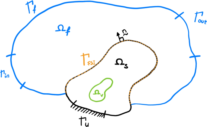
Domain and boundaries of the continuum problem. Symbols are explained in the text
For the remaining boundaries, we denote
- : The inlet boundary of where fluid enters the domain,
- : The outlet boundary of where fluid exits the domain,
- : The remaining boundary of the fluid,
- : The part of the boundary of with constrained displacement,
- : Outward unit normal vector on the boundary of . This normal will be used extensively in the FSI load vector and we thus omit the subscript “s” for .
- : Outward unit normal vector on the boundary of . Note that on , and we thus only use in our derivations of the FSI load vector.
The state variables in our model are the displacement , the velocity , and the hydrostatic pressure . Stationary loads are assumed, so there is no time-dependence in the governing equations. In this work, we use a monolithic (sometimes called unified) approach for the FSI problem, meaning that the state variables are defined over the entire domain . This means that the fluid is able to flow inside solid regions but is restricted by Brinkman penalization (see section 2.1) as illustrated in Fig. 2, and the structural stiffness is also defined everywhere as in normal TO. The equations, however, are not solved in a monolithic fashion, they are solved in a staggered way, i.e., we first solve the fluid equations and then the FSI loads are extracted and used as input for the mechanical problem.
For the design parametrization, we use standard density-based TO Bendsøe and Sigmund (2003) with relative density functions , the optimization variable, and , the physical design, both taking values in [0, 1] at each point in the domain. A value of indicates solid material, while represents fluid or an empty region. Intermediate values in (0, 1) are allowed but undesirable and thus penalized as described below. The physical design is obtained from using a linear PDE-based density filter (Lazarov and Sigmund 2011) with length-scale parameter R. The density filter is followed by the so-called Heaviside projection filter (Wang et al. 2011), with steepness parameter and threshold value , to promote binary-valued, 0-or-1 designs.
The fluid–structure interaction boundary is implicitly defined as a function of the physical design, i.e., , and is used in the evaluation of the FSI load vector in later sections.
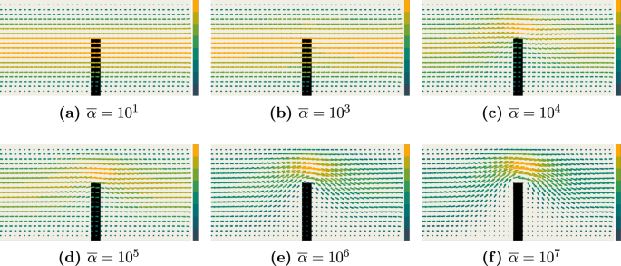
Illustration of the monolithic principle and the influence of the inverse permeability
2.1 Flow problem
The flow is modeled as a viscous incompressible fluid with density and viscosity . It is governed by the stationary Navier–Stokes equations augmented with a Brinkman-term (Borrvall and Petersson 2003) to penalize flow in solid regions. The weak form of the flow problem consists of finding satisfying Dirichlet boundary conditions on the velocity and the integral equation
for all admissible test functions . Here, is a given surface traction, is the symmetric velocity gradient, and the fluid stress is
The coefficient in the Brinkman penalty term in (1) is given by
where q is a penalty parameter and is the flow impermeability. As q decreases, becomes closer to a linear function, which in turn gives a higher resistance to flow in regions with intermediate densities (Borrvall and Petersson 2003). Higher values of reduce the amount of (non-physical) flow through solid parts of the domain (see Fig. 2), but initializing the optimization with too large values may lead to numerical difficulties and increases the likelihood of ending up with a poor solution.
The pressure penalty term in (1) is inspired by Kumar et al. (2020); Kumar and Langelaar (2021). The purpose of this term is to penalize the hydrostatic pressure in solid parts, i.e., in regions where is 1 or close to 1, thus avoiding non-physical propagation of pressure through such parts and pressurized internal holes. In Fig. 1, for example, the domain includes the void region which is not connected to the fluid domain but will be pressurized unless the hydrostatic pressure is penalized. In the numerical examples, the function is taken as the SIMP-like function , with positive constants c and specified in section 6.
Remark
In multiphysics problems (such as FSI) and compressible flow simulations, it can be advantageous to decompose the hydrostatic pressure into a variable component and a constant reference pressure, i.e., . This approach is motivated by the fact that, while absolute pressure influences mechanical loads and material properties, flow dynamics are governed by the pressure gradient, see appendix A for a mathematical derivation. From a numerical perspective, working directly with pressure differences can enhance numerical stability, compared to prescribing large, offsetting absolute pressures at the inlet and outlet. Again, the stationary Navier–Stokes equations are then solved for , and then a constant reference pressure is added to the calculation of the FSI loads, see equation (5) for details.
2.2 Mechanical problem
For the mechanical problem, we assume an isotropic material and stationary, linear elasticity, with a total fluid-load acting on the solid part. According to the principle of virtual work, the displacement should satisfy Dirichlet boundary conditions and
for all admissible test functions . Here, p is again the absolute pressure, defined as . Following the standard SIMP-approach, the stiffness of regions with intermediate densities is penalized. Consequently, assuming an isotropic solid material, the mechanical stress is calculated as
where E is the Young’s modulus of solid material, the positive constant is an artificial stiffness introduced to ensure coercivity of the bi-linear form, is the SIMP-penalty parameter, and is a constant fourth-order tensor depending only on the Poisson’s ratio. An issue with SIMP is the absence of derivative-information when and thus we also investigate the use of Rational Approximation of Material Properties (RAMP), where we substitute with , where is the penalty parameter.
Given (4), Eq. (3) can be rewritten as
From this expression, we infer that if the constant reference pressure is large, then the fluid–structure interaction might occur mainly indirectly, so to speak, via the design.
3 Finite element formulation
In this section, we present the FE formulation obtained by discretizing the continuum problems introduced in Sect. 2. The design variables, flow problem, and mechanical problem are discretized using standard FE techniques, with additional stabilization applied to the flow problem. Particular focus is placed on the FSI load vector, which couples the structural and fluid responses across and requires a detailed derivation and implementation due to its non-standard approximations.
3.1 Discretization of design variables
The relative density functions and are approximated as element-wise constant. The elemental values of , which are denoted , , are collected in , with m being the number of finite elements. Similarly, the physical design has elemental values which are collected in .
As mentioned in Sect. 2, the physical design is obtained from through a combination of PDE-filtering and Heaviside projection, which promotes binary values to more accurately describe the FSI load.
3.1.1 Discretization of the flow problem
The flow problem is discretized using FE approximations for the velocity, , and pressure, . These fields are discretized using hexahedral elements, on which the velocity field is approximated tri-linearly, while the pressure is treated as element-wise constant.
To improve stability, SUPG (Streamline-Upwind Petrov–Galerkin) stabilization is applied to address challenges associated with the convective terms. In our numerical examples, we use box-shaped elements with element-wise constant pressure, so the SUPG stabilization reduces to
where is the domain of element e, and is the stabilization parameter, computed as
with , , defined as in Alexandersen (2023), i.e.,
In some literature, and are defined as and and then taking and in the expression for . However, we found that this could in very rare cases cause numerical issues when the denominator comes very close to 0. Thus, it is recommended to write it as it is written here since there is no risk of division by 0.
Additionally, pressure-jump stabilization (Hughes and Franca 1987; Burman and Hansbo 2007; Thore 2021) is used to avoid oscillations in the pressure field which can occur when using an element-wise constant pressure. The degree of stabilization is controlled by a user-specified parameter .
The residual form of the FE discretized flow problem is expressed as
where the vector collects the FE degrees of freedom for the velocity and pressure, and is the FE load vector arising from the traction load .
3.1.2 Discretization of the mechanics problem
The mechanical problem is discretized using a standard -conforming FE method for linear elasticity. The matrix form of the problem is
where is the stiffness matrix depending on the design , with SIMP-penalization as described by equation (4). Here, collects the displacement degrees of freedom, and represents the FSI load vector. No additional stabilization is required for this problem.
With the exception of the FSI load term, problems (7) and (8) are fairly standard, and we therefore only consider the FSI load vector in detail below.
3.2 Fluid–structure interaction load vector
The FSI load vector is an important part of the FE formulation, as it couples fluid and structural responses across . As mentioned in Sect. 2, it involves contributions from hydrostatic pressure and viscous forces for which the FE approximations are derived separately in the following subsections. These contributions arise from the difference in density between neighboring elements and require integration over element faces.
3.2.1 Discretization
The approximation of the right-hand side of (3) involves integration over the element faces, where contributions from all internal faces in the mesh are accounted for. The design-dependent boundary is approximated by evaluating the jump in across adjacent elemental faces. Thus,
In (9), is the f:th face of element e, with outward normal ; is the number of internal faces of the element; and the factor is introduced since each face is accounted for twice.Footnote1 The density is the density of the neighboring element across face f, and is an increasing function from to . With this construction, if , i.e., element e is solid, and , i.e., element ef contains fluid, we get the FSI load as intended; and when , then the FSI load is zero.
The FE-approximation of the test function, in (9) is on element e given by , with shape function matrix . Here, is the number of DOFs per element, and collects the global DOFs of . The boolean matrix selects the DOFs associated with element e, where is the total number of global DOFs in the system. Substituting the expression for into (9) and splitting the integral on the right, we get
where we used the symmetry of . We now seek an expression for the total FSI load vector, , of the form
where superscript and are used for hydrostatic pressure and viscous forces, respectively. Examining each part of Eq. (10), the goal is to derive an expression for a general element for both FSI load contributions.
3.2.2 Hydrostatic pressure contribution
From (10), the virtual work from the hydrostatic pressure is given by
From this expression, we identify the load vector as
We remark that load vector contributions may be given to DOFs on from internal faces with a node or an edge on . These contributions are then simply zeroed out. The element contributions in (13) are computed as
where the integral of the shape function and face normal is evaluated on a reference element using Gauss quadrature with points , local area scaling , and weights .
3.2.3 Viscous force contribution
The element contribution from the viscous forces is given by
where the term can be written explicitly as
The components of are conveniently obtained from the Voigt-form expression , where is the standard strain–displacement matrix. The velocity gradient multiplied with the normal vector in (14) can now be written as
and then for implementation purposes more conveniently rewritten as
where (not to be confused with the shape function matrix ) contains the components of the normal vector of the current face of the element. Recalling (14) we see that the FSI load contribution from the viscous forces can now be written as
where the integral is evaluated in the same way as for .
4 Topology optimization problems
We consider a fairly general TO problem with a functional associated with flow performance or mechanical performance as objective, and another functional associated with the mechanical performance or total volume as a constraint. The (FE discretized) optimization problem reads
where solves the flow problem (7) for a given design, and solves the mechanics problem (8). In the numerical examples below, parts of the design domain is fixed to solid. This is accounted for by the last constraint which states that elements in should be fixed to be solid in the optimization (this is not implemented as a set of explicit non-linear equality constraints but by simply setting before evaluating the objective and constraints). The velocity and pressure are fixed to zero in .
4.1 Derivatives
The optimization problem (18) will be solved using gradient-based methods. We therefore present derivatives for a general design response g of the form
Assuming that the flow and mechanics state problems are solved exactly, we have
where and are arbitrary vectors. Now we get the derivative with respect to a single physical design variable as
with the Jacobian . Requiring that and solve the adjoint systems
and recalling the symmetry of , (19) gives
The term accounts for explicit design dependency in the Brinkman and pressure penalty terms, as well as the terms in the SUPG stabilization (6).
The second term in the right-hand side of (20b) is computed efficiently as
where , , and is the FSI element load vector. Similarly, the term involving the explicit derivative of the FSI load vector in (21) is computed as
where is slightly more complicated than usual due to the term in (9), which involves the densities of both the current element and its face neighbors. Expressions for the derivatives of the load vector are given in Appendix B.
The complete derivatives are obtained in the standard way using the chain-rule.
4.2 Specialization of functionals
We describe the functionals and in (18) that are available in our code, with the specific choices for each problem detailed in the numerical examples.
4.2.1 Fluid Compliance
Choosing g as the fluid compliance, i.e.,
The fluid compliance is different from the structural compliance in that it tries to maximize the velocity in the direction of the given inlet-traction compared to structural compliance where the goal is to minimize the displacement in the direction of the given loads, hence the minus sign.
The general expression (21), where we can now take the adjoint vector , reduces to
where solves the adjoint system .
4.2.2 Dissipated power
A common objective in the literature on fluid TO is the dissipated power
In matrix notation, we get the functional:
where the factor 1/4 comes from the stiffness matrix being obtained from discretization of .
The derivative is given by (21) with . The explicit part of the derivative is computed as
The velocity-part of the adjoint right-hand side is simply
where the factor 2 comes from the symmetry of and .
4.2.3 Mechanical compliance
Given the FSI load, we get the mechanical compliance as
The adjoint systems (20) become
and
The explicit derivative of g is
By identification, we take as and we get
4.2.4 Maximum total displacement
As an alternative mechanical constraint, we attempt to limit the maximum total displacement, i.e., , with being the Euclidean norm on , in parts of the domain. The max-function is non-differentiable however, so we therefore use a constraint based on the -norm, namely
where and are user-specified constants. The integral is in our numerical examples approximated using the 1-point (the element centroid) Gauss quadrature. The domain is for the valve example in section 6.4 taken as the union of the solid outer shell and the steering pin. As for the gradient (21), the explicit g-derivative is zero. The main complication is the adjoint right-hand side in (20a), but, since , this term can be written as
where the notation indicates that we sum over all elements in . Here, is evaluated in the centroid of element e, and is the volume of element e.
5 Implementation
The code for solving the TO problem (18) is written in C++, based on the code by Aage et al. (2015); see Lundgren et al. (2023, 2024) for additional details. PETSc (v. 3.22.0) (Satish et al. 2025) is used for numerical calculations, and ParaView (v. 5.11.1) (Kitware 2023) is employed for 3D visualization.
To reiterate, the FE discretization employs 8-noded hexahedral elements. The velocity and displacement fields are approximated as element-wise tri-linear and continuous, while the hydrostatic pressure is approximated as element-wise constant. Element integrals are evaluated using standard eight-point Gauss quadrature.
The mechanical state problem (8) is solved using iterative linear solvers, specifically FGMRES with a geometric multi-grid preconditioner.
The flow problem (7) is solved using Newton’s method with linesearch via PETSc’s SNES solver. The linear systems for the Newton search direction are solved using BCGSCL with PETSc’s fieldsplit preconditioner. The relative stopping tolerance for the Newton-solver was set to .
The adjoint problems (20) for both the mechanical and flow problems are solved using the same linear solvers as their corresponding state problems. Relative stopping tolerances are set to for all state and adjoint problems.
The PDE for the linear density filter (Lazarov and Sigmund 2011), being computationally inexpensive, is solved with high accuracy (rtol=) using FGMRES with a geometric multi-grid preconditioner.
As optimization solver, we use the Method of Moving Asymptotes (Svanberg 1987; Aage and Lazarov 2013), with standard parameters for the wall problems and asyinit=0.3, asyincr=1.1, asydecr=0.5 for the valve problem, and with fixed move limits set to 0.2. Following standard practice, the objective and constraints are scaled such that they are of similar magnitude throughout the optimization.