Article Content
1 Introduction
Simulation-driven shape optimization procedures have for several years been studied and applied in a wide range of engineering applications. Most of the designs produced today in automotive, maritime, and aeronautics industries have undergone a certain level of optimization, based on either computational fluid dynamics (CFD) or computational structural mechanics (CSM) simulations. The industrial interest on the field of shape optimization is concurrently accompanied by a significant research effort, see, e.g., Katsapoxaki et al. (2023), Kühl et al. (2022), Upadhyay et al. (2021), Papoutsis-Kiachagias et al. (2019) for some recent publications. The success of such methods in the aforementioned industries naturally raises the question of their applicability in biomedical applications (Marsden 2014). This paper aims to present how several aspects of an optimization method, that are considered established in most fields of engineering interest, can be successfully applied in a biomedical context.
In shape optimization, one searches for the optimal configuration of a domain, so that an objective functional is minimized. A wide variety of optimization methods, ranging from stochastic (or global) (Bäck 1996) to deterministic (or local) (Nocedal and Wright 2006) exists. The decision upon the employment of a specific method depends on the design task and underlying problem. On the one hand, global techniques, such as evolutionary algorithms (Jahangirian and Shahrokhi 2011; Giannakoglou et al. 2006), are able to provide the global optimum, as the name suggests, given that a large number of candidate solutions are evaluated. This option is attractive for non-convex problems and cheap evaluation methods but becomes computationally unfeasible for a large number of control variables and/or expensive evaluation methods. On the other hand, deterministic strategies are able to arrive at a local minimum using the information of the gradient of the objective functional with respect to (w.r.t.) the control, i.e., the shape. These approaches, frequently referred to as gradient-based methods, require support from a tool able to compute the desired gradient. The computation of the gradient is a crucial step that can be realized by several different approaches (Martins and Hwang 2013). Depending on the approach for obtaining the sought gradient, the computational cost of the optimization method can significantly vary. For most applications in the literature, the adjoint method has been the method of choice for the computation of the sought gradient due to its computational efficiency for problems of many control variables, see e.g., Kühl et al. (2019), Papoutsis-Kiachagias and Giannakoglou (2016), Bletzinger (2014), Stück and Rung (2013), Othmer (2008), Brezillon and Gauger (2004).
Regardless of the optimization process to be followed, most of the commonly available methods require the computational modeling of the underlying physical problem. In the case of biomedical applications, this often refers to the numerical solution of blood flows. Numerical simulations based on continuum mechanics can sufficiently describe the flow of blood in an extensive range of applications; see, e.g., Quarteroni et al. (2000) for a review on computational vascular fluid dynamics. The goal of simulating such flows, that within this paper will be referred to as the primal problem, is to predict hemodynamic quantities of interest (QoI). This work considers mechanical hemolysisFootnote1 to be the primary QoI. Hemolysis refers to the mechanical damage of red blood cells (RBCs) and the release of their contents, predominantly hemoglobin, in the blood plasma due to excessively high stress induced by peculiarities of the blood flow. Hemolysis induction is usually encountered in biomedical devices, where large velocity gradients are found, e.g., blood pumps (Yu et al. 2016; Thamsen et al. 2015), but it can also appear in vivo conditions, i.e., in a living person, when vessels delivering blood are kinked or stenosed (Goubergrits et al. 2018). Several computational hemolysis prediction models have been developed and successfully coupled with CFD solvers; see, e.g., Yu et al. (2017) for a review on the topic.
Furthermore, a usual practice in CFD simulations of hemodynamics is to model blood as a Newtonian fluid. While this assumption has been shown to sufficiently describe the rheology of blood in flows exposed to high shear rates, it falls short in flows of low shear rates due to the shear-thinning behavior of blood (Fung 1993). Several non-Newtonian models have been proposed to deal with this inadequacy and account for pseudo-plastic behavior (Quarteroni et al. 2000). Even though most of the available non-Newtonian models cannot account for viscoelastic properties, they can still provide significant information with a small implementation effort into a CFD framework.
An additional aspect of recent biomedical interest is the interaction of blood with a solid surface, which exhibits an increased elasticity. It has been shown that the rigid wall assumption of a classical CFD simulation has in many cases proven to be inadequate to accurately predict certain blood flow problems; see e.g., Hsu et al. (2014), Bazilevs et al. (2010). To this end, extensive focus has recently been given to fluid–structure interaction (FSI) simulations that consider the fluid flow and the displacement of the vessel wall in a coupled manner. A general overview of cardiovascular FSI can be found in Bazilevs et al. (2013).
When a computational model of the physical problem is available, it is common practice to assume precise knowledge of the conditions under which a flow phenomenon occurs. This is, however, rarely the case. Frequently, it is observed that the initial assumption of accurate knowledge is only a coarse approximation, with the actual values fluctuating around what was initially assumed to be precise. If this assumption is employed on a shape optimization procedure, a shape that is considered to be optimal for one application is sometimes proven below par in reality due to the uncertain nature of the conditions under which the application occurs. This led to the emergence of the field of robust shape optimization which aims to identify an optimal solution out of a range of probable conditions. To include the uncertainties in the optimization problem, the uncertain variables, which could refer to, e.g., modeling parameters, boundary conditions, or initial conditions, are considered to follow statistical distributions and are described based on their mean and standard deviation. To this extent, the QoI, that in traditional shape optimization refers to a deterministic quantity, is now affected by the randomness of the uncertain variables and also acts as a statistical quantity, characterized by its statistical moments. The optimization is then usually formulated as the minimization of functionals combining these moments, depending on the design task. The identification of the statistical moments of the QoI is referred to as Uncertainty Quantification (UQ). The most straightforward strategies for UQ refer to Monte Carlo (MC) (Janssen 2013) or MC-based methods (Chatterjee et al. 2019; Morokoff and Caflisch 1995), where the simulation of an excessive number of realizations, i.e., specific outcomes of the random process, is required. To avoid the computationally intensive simulation of several realizations, the Method of Moments (MoM) has been proposed as a suitable alternative for UQ (Kranz et al. 2023; Papadimitriou and Giannakoglou 2013). The MoM is based on a Taylor series expansion of the QoI around the mean values of the uncertain variables and can provide the sought statistical moments with the use of derivatives of the QoI w.r.t. the uncertain variables. The first-order second-moment (FOSM) method truncates the expansion after the first-order term. It is worth noting that the FOSM method requires no assumption on the type of distribution of the uncertain parameters (Kriegesmann and Lüdeker 2019).
In this paper, we present the gradient-based robust shape optimization of an idealized bypass graft, frequently used in surgical procedures as an alternative route around severely stenosed arteries. Studies such as those of Jiang et al. (2016) and Zhang and Liu (2015) have previously investigated the deterministic shape and topology optimization, respectively, of idealized two-dimensional bypass configurations using the level-set method in combination with adjoint techniques for the minimization of a blood damage-related metric. In both studies, significant improvements were identified as compared to initial configurations, highlighting the potential of formal optimization techniques for arterial graft design. It is also worth noting the recent study of Habibi et al. (2025), in which an automatic multi-objective Bayesian shape optimization was built for patient-specific vascular grafts. Similarly to the present work, the authors of Habibi et al. (2025) built their optimization framework based on steady-state CFD simulations and later assessed their designs on transient simulations, under the rigid wall assumption. They noted that in most of the cases, the steady-state produced shapes also showed superior results when assessed by transient simulations. The optimization procedure followed in this work considers the control to be the complete three-dimensional shape of the graft and host artery, in a CAD-free manner (Radtke et al. 2023). Modeling parameters for the estimation of hemolysis (3 parameters) and non-Newtonian viscosity (4 parameters) are considered uncertain, cf. Eq. (8). The optimization targets the minimization of the convex combination of the first two statistical moments of the QoI. Shape sensitivities are computed using the continuous adjoint method, developed and presented in Bletsos et al. (2023, 2021). The MoM is employed for the UQ of the problem. Select optimized shapes are subsequently assessed by means of a partitioned FSI approach.
The remainder of this paper is organized as follows: In Sect. 2, we present the numerical methodology employed for the solution of the robust shape optimization problem. Specifically, we describe each step of the process as well as numerical aspects to arrive at the necessary quantities for optimization. The section closes with the presentation of the complete optimization algorithm. Section 3 is concerned with the application of the presented methodology on the idealized bypass graft geometry. We perform five optimization runs by combining different uncertain parameters and weights in the definition of the robust objective functional. Two selected designs are further evaluated under FSI conditions. The paper closes with conclusions and outlines future work directions in Sect. 4. In “Appendix A”, we briefly describe the FSI methodology employed in this work. “Appendix B” presents core aspects of the derivation process of the continuous adjoint system employed in this work and a verification study for the proposed adjoint sensitivity expression. “Appendix C” presents a sensitivity analysis study w.r.t. the uncertain parameters.
Throughout the paper, Einstein’s summation convention applies for repeated lower-case Latin subscripts. Vectors and higher-order tensors are defined with reference to Cartesian coordinates.
2 Methodology
This section is dedicated to the presentation of key aspects of the numerical method employed in this work. Specifically, we present the primal problem and discuss its numerical solution using CFD. The primal problem is subsequently considered uncertain by means of its parameters and we discuss the UQ method followed to identify the statistical moments of the QoI. The section closes with the presentation of the robust shape optimization problem in the framework of a CAD-free gradient-based optimization approach.
2.1 Blood flow modeling
In what follows, we refer to the fluid domain as and its boundary as . Furthermore, we distinguish segments of the boundary as inlet, , outlet , and wall , with . We model blood as an incompressible, non-Newtonian fluid and the flow as laminar and steady-state. The equations of state are thus described based on the conservation of mass and momentum in , viz.
where and refer to the residual forms of the continuity and momentum equations, respectively. We denote with the Cartesian spatial coordinate, denotes the fluid’s density, the Cartesian velocity components, p the pressure, the strain-rate tensor components, and the Kronecker delta components. The effective viscosity of the non-Newtonian fluid is given based on a non-linear relation to the second invariant of the strain-rate tensor, which we define as
In this work, we employ the Carreau model to describe this relation, viz.
where , n, , and are considered as parameters of the model. The Carreau model appears to be one of the most suitable choices for the investigations conducted in this study, as it effectively supports the continuous adjoint calculus and spans a broad range of viscosity values. However, it must be noted that the choice of the non-Newtonian viscosity model is not restrictive and other models able to describe the shear-thinning nature of blood, such as the Power-law (Shibeshi and Collins 2005), Casson law (Blair 1959), and modified Cross model (Zhang and Liu 2015), could be used.
Equations (1, 2, 4) describe the flow of blood. In addition to this, we also model hemolysis based on a typical power-law hemolysis prediction model, which is one-way coupled to the flow equations (Garon and Farinas 2004; Giersiepen et al. 1990). The one-way coupling implies that information from the solution of the flow dynamics are used by the hemolysis model with no subsequent retro-action to them. In an Eulerian framework, this can be written as
where is the unknown variable and H denotes a local measure for the released hemoglobin to the total hemoglobin within an RBC. Hemolysis induction is governed by shear stresses and the model is driven by that is based on the second invariant of the stress tensor, viz.
It is noted that for an incompressible fluid and thus disappears on a converged state of the flow. The model is closed by a set of parameters .
Once the flow solution and distribution of is known, a QoI that measures the hemolysis induction potential of the flow can be computed. A usual metric for this QoI is a hemolysis index that measures the mass-flow-average of hemolysis on the outlet of the computational domain
The boundary conditions employed to close the flow and hemolysis problem are as follows:
- Dirichlet velocity and hemolysis and zero Neumann pressure on ,
- Dirichlet velocity and zero Neumann pressure and hemolysis on ,
- Dirichlet pressure and zero Neumann velocity and hemolysis on .
The numerical solution of the primal problem is based on the finite volume method employed by the in-house software (Rung et al. 2009). For the solution of Eqs. (1, 2), the segregated algorithm employs the SIMPLE method for pressure–velocity coupling. A collocated storage arrangement is employed for all transport quantities and parallelization is possible by means of domain decomposition (Yakubov et al. 2013). For the non-Newtonian fluid model employed in this work, the non-linear relation of the effective viscosity to the strain-rate tensor, cf. Eq. (4), introduces an additional non-linearity to the momentum equations. This is resolved in our numerical scheme based on a Picard-like linerization approach, in which the effective viscosity is evaluated at each cell center based on the velocity of the previous pressure–velocity coupling iteration. The face-based values of viscosity required for the discretization of the diffusive term are obtained based on a linear interpolation from the adjacent cells. Once Eqs. (1, 2) are solved, Eq. (5) can be solved in a straightforward manner using similar discretization techniques. In this work, the higher-order QUICK scheme is used to discretize all convective terms.
For the FSI simulations considered in this work, the fluid solver needs to be coupled to a structural solver. Key aspects of the partitioned solution approach followed for FSI in this work are presented in “Appendix A”. The interested reader is pointed to Bletsos et al. (2024) for detailed information.
2.2 Uncertainty quantification based on the MoM
The parameters employed by the hemolysis and non-Newtonian models are typically deduced from fitting models to experimental data. Although experiments are conducted under well-controlled conditions, the same parameter sets are frequently used for more complex computational studies. Furthermore, it is often the case that experimental studies result in a different fitting of the same models thus proposing a different set of parameters; see, e.g., Zhang et al. (2011), Giersiepen et al. (1990), Heuser and Opitz (1980) as regards the hemolysis parameters. While this discrepancy can be significant on the predictive quality of the computational model itself, it can also lead to unfavorable results when optimization is considered. To avoid additional cumbersome and often unfeasible experiments, this work proposes to approximate these parameters as uncertain variables. To this extent, we consider
as two independent dimensional vectors of uncertain variables, with and for the case of hemolysis and non-Newtonian parameters, respectively. Each uncertain variable is associated with a probability density function resulting in corresponding vectors of mean values and standard deviations, denoted as and , respectively. For the sake of brevity, the superscript of the previously defined vectors is dropped in what follows and only specified when necessary.
Since the primal problem is now dependent on a number of uncertain variables, so is the QoI, i.e., . We consider the propagation of the uncertainties to the QoI based on the FOSM method, which develops the QoI based on a truncated first-order Taylor series expansion around the mean values of the uncertain variables, viz.
Assuming that the covariance matrix of the uncertain variables is diagonal, it can be shown based on expression (9) that the first two statistical moments of the QoI can be approximated as
see, e.g., (Kriegesmann and Lüdeker 2019). Based on FOSM, the mean of the QoI can be approximated by one computation at , while the variance requires in addition the derivatives of the QoI w.r.t. the uncertain variables for . Note, however, that the estimation of both statistical moments is independent of the underlying probability density function of the uncertain variables and only requires the mean value and variance (standard deviation) vectors to be chosen by the user.
In comparison to other UQ methods, e.g., based on Monte Carlo techniques, the FOSM method allows the evaluation of the sought statistical moments of the QoI and their derivatives at a reasonable number of primal/adjoint evaluations per shape update, as illustrated in Sect. 2.3.4. Furthermore, it decouples the optimization process from the requirement of specifying a probability density function, which can be ambiguous because of insufficient relevant experimental data due to the nature of the problem. Higher-order methods of moments, e.g., the second-order second-moment (SOSM) method (Papoutsis-Kiachagias et al. 2012), increase the necessary computations, because higher-order derivatives need to be evaluated. The FOSM method avoids this and is by construction sufficiently accurate when the QoI is approximately linear in a neighborhood close to the selected mean value of the uncertain variables. To this end, we present a sensitivity analysis study w.r.t. the uncertain variables in “Appendix C”.
This work considers a low number of uncertain variables and is therefore computationally reasonable to approximate the derivatives of Eq. (11) based on the finite differences method, viz.
Note that only a first-order accurate finite differences scheme is considered, since a similar first-order assumption is already made in the construction of the method, cf. Eq. (9). The determination of Eq. (12) requires M additional simulations. However, it is worth noting that in the case of uncertain hemolysis parameters, the determination of the QoI does not require the recomputation of the flow field but only the computation of the hemolysis equation due to the one-way coupling assumed between the flow and the hemolysis equation. The numerical solution of the latter is significantly faster than the solution of the flow field and therefore the cost of computing Eq. (12) can be considered negligible. For the uncertain non-Newtonian parameters, even though the flow field needs to be recomputed to estimate the perturbed QoI, the numerical method can be warm-started from the flow field of the unperturbed state, since the topology of the computational mesh is the same. Therefore, in both cases, the computational cost of the M additional simulations required for the estimation of Eq. (12) is significantly smaller than M CFD solutions.
2.3 Robust shape optimization problem
Let denote an objective functional that depends exclusively on a state and a control , where Y, U denote the Banach spaces of state and control, respectively. We assume that the state is unique on and thus the control to state mapping exists. Therefore, one can consider a reduced objective functional . Practically, the above statements mean that given a specific control , the objective functional is determined through the, now hidden, solution of the state equations. The goal of a deterministic optimization problem is to minimize the (reduced) objective functional by updating the control until is sufficiently approximated, for which , where denotes a neighborhood of .
Consider now that the state, initially assumed to depend only on the control and the underlying physics (state equations), is unpredictably perturbed due to reasons unrelated to the control, e.g., due to an inconsistent/simplified modeling of the physics resulting to a false estimation of the state. The solution found by the deterministic problem is likely not to be optimal anymore. The resolution of this discrepancy is addressed by robust optimization, in which a certain level of uncertainty is prescribed to select modeling parameters. The goal of robust optimization is not to arrive at a set of optimal solutions for each probable state but rather to arrive at a control that likely performs better than the initial for each probable state, that is expressed by the mean of the QoI. At the same time, the optimization should target at a shape that exhibits minimum variations on its performance w.r.t. the uncertain input, which is expressed by the standard deviation of the QoI. To this end, the objective functional is considered as a statistical quantity. The optimization targets the minimization of its statistical moments rather than its value at each probable state, viz.
where and correspond to the mean value and standard deviation of a QoI, respectively, and denote weights to be chosen before the optimization starts.
In this paper, we consider the control to be associated with the shape of our geometry and to be of deterministic nature, i.e., not subject to uncertainties. Therefore, one can express the objective functional as , where in accordance to Sect. 2.2, stands for an uncertain variable vector that implicitly acts on the objective functional (13) through its influence on the state. We are interested in optimizing the shape based on a gradient-based method and we therefore require
which based on the UQ approach followed herein [see Eqs. (10, 11)] can be expanded as
where the vector is defined as
The determination of Eq. (15) requires the computation of , and at . The computation of the derivatives w.r.t. the uncertain variables is addressed in Sect. 2.2.
2.3.1 Determination of first-order derivative w.r.t. the control
We are interested in applying a parameter-free shape optimization method, which means that instead of controlling the shape through a finite number of parameters, e.g., control points of B-splines (Farhikhteh et al. 2023), the complete shape or rather the discrete representation of the shape is considered as the control. To this extent, the number of control variables can be in the order of and derivative computation methods that scale with the number of control variables, e.g., finite differences, are unfeasible.
Therefore, the continuous adjoint method is employed for the determination of the sought first-order derivative w.r.t. the control. The adjoint (dual) to the primal problem described in Sect. 2.1 reads
Adjoint velocity components and pressure are denoted by and , respectively. Adjoint hemolysis is denoted by and adjoint viscosity is denoted by , while stands for the adjoint strain-rate tensor components. Tensors and relate to the primal hemolysis and non-Newtonian models, respectively, and for the specific models employed in this work can be computed based on
The boundary conditions employed to close the adjoint field equations are as follows:
- Zero Dirichlet adjoint velocity and zero Neumann adjoint pressure and adjoint hemolysis on and ,
- Dirichlet adjoint pressure, adjoint hemolysis, and adjoint tangential velocity components based on
(22)(23)(24)
where a superscript t implies the tangential components of a vector and a subscript n implies the normal to the surface component of a vector, i.e., with denoting the normal vector. The normal component of adjoint velocity is approximated by satisfying adjoint continuity, Eq. (17), on the outlet.
The resulting system of field adjoint Eqs. (17-20) and their corresponding boundary conditions is derived by extension of the derivations presented in Bletsos et al. (2023, 2021) to consider cross-coupling terms between primal hemolysis and non-Newtonian viscosity equations. Key aspects of the derivation process of the employed adjoint system can be found in “Appendix B”. Note that in the FOSM approach, the sought derivative must be computed at the mean values of the uncertain variables. Therefore, in the context of uncertain hemolysis or non-Newtonian parameters, the computation of the primal and adjoint systems is realized for or , respectively.
Once the primal and adjoint equation systems are solved, the sought derivative can be computed based on
where denotes the vector of face areas of the discretized wall boundary.
Similar to the primal state equations, the numerical solution of their adjoint counterparts is based on the finite volume method employed by . It is interesting to note that similar to its primal counterpart, the adjoint hemolysis equation (19) is again one-way coupled to the adjoint flow equations (17,18), but this time the coupling direction is reversed. This implies that adjoint hemolysis is required for the solution of the adjoint flow equations with no retro-action to it. From a numerical point of view, this allows us to independently solve the adjoint hemolysis equation based solely on information from the primal solution. Tensors and require only primal flow information and can thus be computed once, before the solution of any adjoint equation. The adjoint pressure–velocity coupling is resolved by a similar to the primal SIMPLE algorithm. Note that in adjoint systems, the information transfer is reversed w.r.t. to the primal. To this end, the convective terms are discretized by the downwind analogy of QUICK. The diffusive term is self-adjoint, and thus, the same discretization schemes as in the primal can be employed. The remaining terms in adjoint momentum, stemming from hemolysis and non-Newtonian properties, are treated as source terms. Similar to its primal counterpart, adjoint viscosity is computed by means of an explicit approach where the adjoint velocity components of the previous adjoint pressure–velocity coupling iteration are employed in Eq. (20). Due to the algebraic nature of the adjoint viscosity equation, no boundary conditions are required. When adjoint viscosity is required on a boundary face, its value is extrapolated from the adjacent cell center.
2.3.2 Determination of second-order mixed derivative
The computation of Eq. (15) requires the estimation of the mixed second-order derivative of the QoI w.r.t the control and the uncertain variables. While the computation of second-order derivatives can in general be a cumbersome task, Eq. (15) does not require the explicit computation of the mixed second derivative but instead its projection on the vector, as noted by Fragkos et al. (2019) and Krüger et al. (2023). This alleviates some of the computational effort, since the projection can be efficiently computed based on an additional adjoint system, as suggested by Fragkos et al. (2019), or by an efficient finite differences method, as suggested by Krüger et al. (2023). The finite differences approach is followed herein. The interested reader is pointed to the original paper for further details.
The sought projected derivative can be computed to second-order accuracy based on
The essential difference between expression (26) and a classic finite differences method is that while the latter needs to perturb each individual uncertain variable while keeping the rest constant, the former can approximate the sought quantity by perturbing the complete vector of mean values simultaneously. Therefore, instead of the 4M additional simulations that would otherwise be required for the approximation of the second-order mixed derivative, the projected quantity can be approximated to second-order accuracy with 4 additional simulations, i.e., 2 primal and 2 adjoint simulations at and . The value of the perturbation size is , where is fixed as the authors of the original publication suggest.
2.3.3 Determination of descent direction
In parameter-free shape optimization, the computation of the shape sensitivity, i.e., Eq. (15), is not sufficient to optimize the shape. An in-depth mathematical explanation of this restriction can be found in Allaire et al. (2021). In practice, we are interested to update the shape and the corresponding mesh of the domain without the need of re-meshing. To this extent, we are searching for a deformation field that can sustain, as much as possible, the quality of the mesh, so that the optimization process can continue uninterrupted. Therefore, a descent direction (deformation) field over the design surface is sought and it must be sufficiently smooth, so that each shape update results in feasible solutions in which one can numerically solve the primal and adjoint equations. This topic is extensively discussed in the recent publication Radtke et al. (2023).
A variety of methods exists to identify such a descent direction. A gross classification can be made depending on the number of additional steps required after the approximation of the shape sensitivity. On the one hand, methods such as sensitivity filtering (Kröger and Rung 2015) or the, frequently called, Laplace–Beltrami method (Vassberg and Jameson 2006), compute a deformation field on the shape of the domain. Subsequently, another step needs to be taken to propagate the field to the interior nodes. On the other hand, methods like the Steklov–Poincaré (Welker 2016) or the p-Laplace (Müller et al. 2021) are able to compute the deformation field in the complete computational domain in one step. Based on this and since the p-Laplace method requires a much larger computational effort due to its highly non-linear character, this paper employs the Steklov–Poincaré method.
The descent direction field is thus computed based on
where corresponds to a diffusivity coefficient. Herein, it is set to the reciprocal of the distance from the nearest wall boundary. The quantity s refers to the local shape sensitivity of the discretized shape and corresponds to dJ/du for a boundary face on . The solution of Eq. (27) is realized via the finite volume discretization for a diffusive term and the field is computed on the cell centers. The mesh update is then realized by a Shepard’s interpolation (Shepard 1968) of the cell-centered descent direction to the nodal positions of the mesh. Schematically, this is illustrated for a node by and it implies the inverse distance weighting interpolation strategy from all cells in which the node exists. Once the nodal deformations are available, the mesh can be updated based on
for all nodes of the mesh. Here, denotes the position vector of a node, denotes a constant step size, and the superscript i denotes the optimization iteration index.
2.3.4 Optimization algorithm
The adjoint-assisted optimization algorithm for the FOSM-based robust shape optimization problem is presented in Algorithm 1. Initially, the uncertain variables are set to their mean values and the primal problem is solved (line 2). Then, a primal problem is simulated for each uncertain variable, in which it is perturbed, while the remaining are fixed to the mean values (line 4). Based on these simulations, the mean value and standard deviation of the QoI can be calculated. The algorithm then checks for convergence by comparing the relative change of the objective from one step to the other (line 7). If convergence is not achieved, an adjoint problem is solved for uncertain variables set to their mean values (line 10). For the determination of the second-order mixed derivative, all uncertain variables are simultaneously perturbed by and the corresponding primal and adjoint problems are solved (lines 12,13). The sensitivity is then calculated (line 15) and passed as input to the descent direction computation (line 16). Once this is computed, each numerical node is updated (line 17) and the optimization continues to the next step.
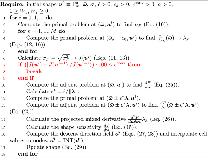
FOSM-based robust parameter-free shape optimization algorithm using the adjoint method.
Note that the presented algorithm distinguishes between statements with the keyword “Compute” and “Calculate”. The former can require substantial computational resources, since it relates to primal or adjoint CFD simulations or the computation of the descent direction, while the latter requires trivial resources for the determination of the sought quantities. Furthermore, it is worth noting that the computations in line 4 can be trivially parallelized, since they are independent of each other. The same holds for the primal simulations in line 12 and the subsequent corresponding adjoint simulations in line 13. Overall, one shape update requires CFD simulations. However, it must be noted that in addition to the trivial parallelization possibility in several stages of the algorithm, the cost of the M simulations related to the loop in lines 3–5 is significantly lower to the cost of full CFD simulations. The finite differences conducted therein require only the perturbation of the mean uncertain variables. Therefore, in the case of uncertain hemolysis parameters and due to the one-way coupling of the hemolysis model with the flow equations, the main flow solution, which is already available from line 2 of the algorithm, can be used to arrive with trivial resources in the sought derivative. In the case of uncertain non-Newtonian parameters, the flow equations need to be recomputed; however, the simulation can be warm-started from the solution of the unperturbed flow, thus resulting in a significant speed-up of the M additional simulations. To highlight this, we present Fig. 1, which shows the wall clock time for the first (initial shape) primal simulation and for the computations in lines 3–5 of the algorithm. The results shown therein refer to the case studied in Sect. 3. All computations are parallelized using 90 CPUs.
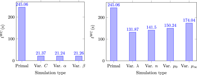
Idealized arterial bypass graft (Sect. 3): wall clock time required for primal problem solution and perturbed primal problem, lines 2 and 4 (Algorithm 1), respectively. Left: uncertain hemolysis parameters Right: uncertain non-Newtonian parameters
Note that in the case of uncertain hemolysis parameters, the wall clock time of the computations in lines 3–5 are significantly faster, since the primal flow is already resolved and due to the one-way coupling, as outlined above. In addition, all perturbed primal simulations can be performed in parallel. This would make the computational cost of the loop in lines 3–5 approximately equal to the cost of the slowest simulation, e.g., based on Fig. 1, and for the uncertain hemolysis parameters and non-Newtonian parameters, respectively.
3 Applications
The 3D geometry studied in this paper refers to an idealized arterial bypass graft. An arterial bypass graft is a segment of a healthy (biological or artificial) blood vessel that is used to divert blood around narrowed or occluded parts of an impaired artery. A sketch of the initial geometry is shown in Fig. 2. The diameters of the bypass graft and the artery are set to and , respectively. The size of the idealized impaired artery geometry is chosen, so that it approximately matches a common iliac or femoral artery (Wazzan et al. 2022).
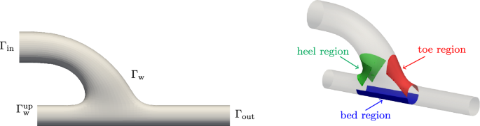
Sketch of the initial idealized geometry of the arterial bypass graft. Left: side view of the geometry annotated with the boundary patches. Right: perspective view of the geometry annotated with the critical regions of the anastomosis
An extensive FSI and CFD qualitative study was performed on this geometry in Bletsos et al. (2024). Therein, it was identified that the shape of the anastomosis, i.e., the connection between the implant and the impaired artery, is one of the most critical parameters in which one can intervene for the hemodynamic response of the implant. Based on this finding and considering its clinical relevance, this paper is motivated to formally optimize the shape, i.e., in contrast to the parametric study conducted in Bletsos et al. (2024), based on the methodology presented in Sect. 2.
3.1 Primal simulation setup
The reproducible process for the discretization of the computational domain is thoroughly described in Bletsos et al. (2024) and results in a block-structured mesh of 315k control volumes. The boundary patch is considered as a wall boundary, thus mimicking a complete occlusion of the impaired artery.
The shape optimization problem considers steady-state flow conditions. However, the steady inflow is chosen based on the peak volume flux of a suitably scaled flow pulse for a patient in rest conditions (Wilson et al. 2005). The choice of performing the optimization at the peak volume flux is made based on the anticipation of maximum hemolysis induction potential at this condition. The flux is then redistributed along the inlet based on a Poiseuille velocity profile, as shown in Fig. 3.
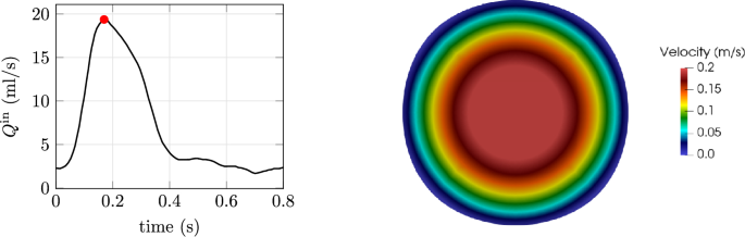
Left: volume flux for rest conditions marked by a red point at the time instant in which the steady-state optimization studies are performed. Right: velocity profile at the inlet based on the prescribed volume flux
The prescribed flux is and amounts to a Reynolds number of
and denoting the Newtonian viscosity of blood in high shear rates. Based on the prescribed flow conditions, an average dimensionless near-wall spacing from the walls is estimated at . Furthermore and due to the employed rigid wall assumption, a zero pressure is prescribed at the outlet of the computational domain. The fluid is modeled as non-Newtonian and the viscosity computation is based on the Carreau model, cf. Eq. (4).
3.2 Optimization setup
The optimization studies consider the complete boundary section to be subjected for design, while is bound to its initial configuration. Furthermore and as discussed in Sect. 2, the hemolysis or non-Newtonian parameters are considered to be uncertain. To this end, each uncertain variable is associated with a mean value and a standard deviation.
3.2.1 Uncertain hemolysis parameters
In this case, the non-Newtonian parameters are fixed to the Carreau parameters, i.e., , , , . The vector of uncertain parameters is then defined as
The hemolysis parameters appearing in Eq. (5), which are deduced from data-fitting experimental results from fully controlled configurations, see, e.g., Giersiepen et al. (1990), are here considered uncertain. The mean value and standard deviation vectors are prescribed as
The choice of is made based on the frequency that this set of parameters is used in computational studies in literature; see, e.g., Yu et al. (2017), Thamsen et al. (2015). We note that this choice is ambiguous and, therefore, the results presented in this study are discussed in a qualitative manner rather than quantitative. The standard deviations are selected under the assumption of a normal distribution, such that parameter sets proposed in the literature fall within approximately . This corresponds to a 95.4% confidence interval, reflecting the belief that these values represent typical variability. Additionally, the prescribed mean and standard deviation vectors assure that the probable space (99.73 % probability for a normal distribution) does not include non-physical solutions such as .
3.2.2 Uncertain non-Newtonian parameters
In this case, the hemolysis parameters are fixed to the set of parameters employed as in Eq. (32). The vector of uncertain variables is defined as
In this case, the parameters employed to model the non-Newtonian viscosity of blood in Eq. (4) are considered uncertain. These parameters are, similarly to the hemolysis parameters, deduced by fitting experimental data. The mean value and standard deviation vectors are prescribed as
Based on the employed mean and standard deviation vectors and by assuming underlying normal distributions for each uncertain variable, Fig. 4 shows the probable (within 95.4% of each uncertain variable probability) space in which viscosity could be represented.
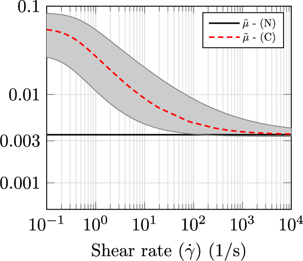
Newtonian (N) and non-Newtonian viscosity (C), based on the Carreau model. Gray area denotes the range in which viscosity is most likely (95.4% probability) to be represented based on the employed and
As shown, the choice of and does not allow for non-physical solutions, e.g., negative viscosities, and sustains necessary characteristics of a blood non-Newtonian model, such as converging to an experimentally measured constant viscosity at high shear rates.
3.2.3 General optimization parameters
For both cases of uncertain modeling parameters, optimization studies are performed for different sets of weighting parameters (), cf. Eq. (13). Specifically, optimizations are performed for
- () = (1, 0) denoted as “DET”,
- () = (0.5, 0.5) denoted as “MIXED”,
- () = (0, 1) denoted as “STD”.
Note that based on our setup, the DET optimization is identical for both uncertain hemolysis and uncertain non-Newtonian parameters.
Additionally, the perturbation size employed in the finite differences computation of the first-order derivative of the QoI w.r.t. the uncertain variables (Eq. (12)) is set to approximately three orders of magnitude smaller than each mean value of the perturbed uncertain variable. The dynamically changing perturbation size for the projected second-order mixed derivative is computed based on . Convergence is monitored by . We note that this corresponds to a very strict convergence criterion but might allow us to explore additional shapes in the optimization sequence. Usual choices would refer to ; see, e.g., Radtke et al. (2023). However, due to the increased computational cost of a robust shape optimization method in comparison to a deterministic one, we also apply as a stop condition the maximum number of optimization iterations, which for the study at hand is set to 230, based on our computational capabilities. The fixed optimization step size is implicitly determined on the first optimization iteration by a maximum displacement approach, that is
which scales the descent direction computed by Eqs. (27, 28), so that the maximum applied deformation on the first optimization iteration is equal to .
The QoI F, the statistical moments of which we want to minimize, is the hemolysis index defined in Eq. (7).
3.3 Results
The results are presented for each set of uncertain variables separately. A discussion is then included on the collective results of the optimization studies. Selected designs are then subsequently evaluated by FSI simulations.
3.3.1 Uncertain hemolysis parameters
Figure 5 shows the FOSM-estimated decrease of the mean value and standard deviation of the QoI for the three optimization cases with uncertain hemolysis parameters. As shown therein, all cases manage to minimize the mean by more than 35%, even though the STD case does not explicitly involve the optimization of the mean in the formulation of the problem. As expected, the DET case leads to the highest estimated decrease of approximately 52%. Specifically for the DET case, the mean value of the QoI is decreased from to and the standard deviation from to . Furthermore, we present in Fig. 6 the relative change of the objective functional in percent for two subsequent shapes in the optimization history. As shown there, all methods manage to arrive at a relative change smaller that 0.2%, which is, however, significantly larger than the employed threshold. This convergence can be accelerated by an increase of the employed step size. Interestingly, the DET optimization case outperforms the other two in the decrease of the standard deviation as well, even though it does not explicitly account for its minimization. This result indicates an inherent robustness of the case w.r.t. the hemolysis parameters. In view of these findings, the shape produced by the DET procedure is deemed as the general optimal solution out of the three. To this extent, it is further scrutinized w.r.t. the statistical moments of the QoI.
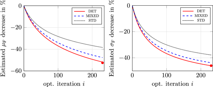
Optimizations for uncertain hemolysis parameters. Left: FOSM-predicted decrease of the mean value of the QoI. Right: FOSM-predicted decrease of the standard deviation of the QoI. Filled circles denote the MC-predicted mean value and standard deviation decrease for DET (see Fig. 7)
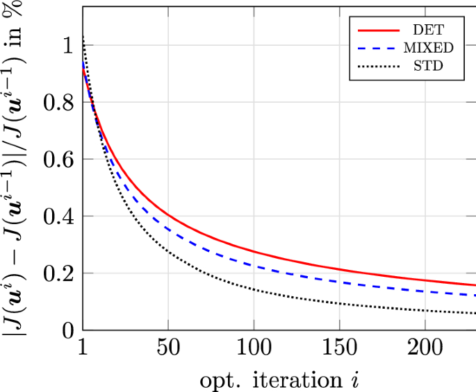
Optimizations for uncertain hemolysis parameters. Relative change of the objective functional in percent for two subsequent shapes
The FOSM method considers a linear relation between the QoI and the uncertain parameters. To evaluate the accuracy of this prediction throughout the optimization, additional MC simulations with a total sample size of are realized for the initial and optimized (DET) shapes. The samples are randomly selected using a normal distribution, for each uncertain variable, with a mean and standard deviation as the one employed by the FOSM-based optimizer. The results of the MC studies are shown in Fig. 7. The FOSM-predicted mean values of the initial and optimized shapes differ from the MC prediction by less than 6%. The standard deviation predictions differ by approximately 14%. Nevertheless, the underprediction of the statistical moments by the FOSM method is consistent for both initial and final shapes, thus resulting in an excellent prediction of the relative decrease of the statistical moments during the optimization process, as illustrated by the filled circles in Fig. 5.
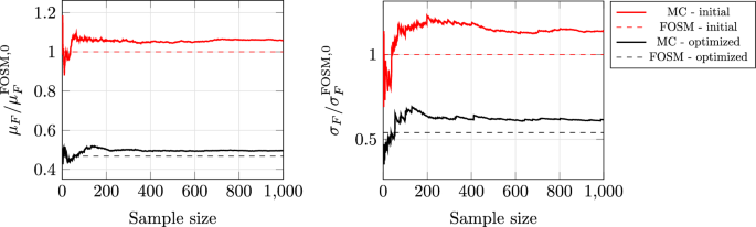
MC study for uncertain hemolysis parameters. Left: running mean value of the QoI for the initial shape (red continuous line) and the optimized shape produced by DET (black continuous line) computed by the MC procedure with . Right: running standard deviation of the QoI. Dashed lines denote the FOSM-predicted statistical moments for reference. Results are normalized by the FOSM-predicted mean value and standard deviation of the initial shape accordingly
Furthermore, it should be noted that based on the employed step size, all optimizations terminated due to the maximum iteration limit. Even though a small step size, as the one employed in this work, can slow down the optimization process, it guarantees that the process can continue uninterrupted. As discussed in Sect. 2, we employ a parameter-free shape optimization approach in which the deformation of the shape is realized directly on the level of the mesh. It is therefore important to the process that the meshes produced in the sequence sustain a certain level of their initial mesh quality. One of the ways to guarantee this property during the optimization is to employ a relatively small step size.
3.3.2 Uncertain non-Newtonian parameters
Figure 8 shows the FOSM-estimated decrease of the statistical moments of the QoI for the three optimization cases with uncertain non-Newtonian parameters. Two observations of interest can be made for these results. First, it is shown that all three cases lead to a very similar optimization history w.r.t. the mean value of the QoI. Second, as regards the standard deviation relative decrease prediction, it is shown that the STD procedure shows the most prominent decrease in accordance to our expectations, since it targets exclusively the minimization of the standard deviation of the QoI. Specifically, the final shape obtained by the STD procedure results in approximately 43% decrease of the standard deviation of the QoI, while the DET procedure terminates at a decrease of approximately 40%. It is also interesting to note that the MIXED optimization run terminates abruptly after 172 optimization iterations due to mesh deformations that heavily deteriorated the quality of the grid, thus leading to the divergence of the primal solver. As in the case of uncertain hemolysis parameters, Fig. 9 shows the relative change of the objective functional. A similar convergence history is noted as in Sect. 3.3.1, with fluctuations, however, noted in the STD case. Overall, the results of the optimization runs suggest that the shape produced by STD exhibits the most beneficial behavior for both monitored statistical moments. In specific, the STD case managed to reduce the mean value of the QoI from to and the standard deviation from to . To this end and similar to the case of uncertain hemolysis parameters, the shape produced by the STD procedure is further evaluated through an MC study with a sample size of .