The optimization of seismic designs by metaheuristic algorithms is a field of research that has gained significant interest in recent years. Proof of this is the growing number of papers published on the subject where the seismic design of buildings is optimized (Joyner et al. 2021; Rafiei Mohammadi et al. 2024), existing buildings are upgraded through optimal distribution of protective technology (Moghaddam et al. 2022), or annual repair costs associated with earthquakes are minimized (Ghasemof et al. 2022). Most of the interest shown by the scientific community in optimizing seismic designs is because these techniques increase the resilience and sustainability of infrastructure, which is in tune with the ninth and eleventh sustainable development goals set forth by the United Nations (2021).

Despite the numerous academic examples of seismic optimization using metaheuristics found in the literature, it can be said that the practical use of optimization algorithms in the field of earthquake or structural engineering is extremely uncommon. One aspect that discourages designers from using metaheuristic optimization in their professional practice is the long execution time of these algorithms (Xiao et al. 2022). Depending on the characteristics of the metaheuristic, the problem to be solved, and the computer equipment, a single run of an optimization algorithm can easily take several days. One strategy that has proven effective in reducing the computational cost of optimization processes is the use of surrogate models, which can be simplified analysis methods (Mokarram and Banan 2018) or predictive mathematical models such as artificial neural networks (ANNs) (Lagaros and Papadrakakis 2004).

The objective of this work is to explore the applicability of ANNs to reduce the computational cost of optimizing the retrofit of a mid-rise reinforced concrete frame equipped with buckling-restrained braces (BRBs) subject to soft soil earthquake ground motions. Nonlinear time history analysis (NTHA) was used to evaluate the generated designs because, given their highly nonlinear behavior, the dynamic response of BRB frames can only be accurately described by this kind of analysis. A mid-rise building was chosen as case study example because this type of structural systems is one of the most common in cities worldwide (Arteta et al. 2019). The optimization process was executed through simulated annealing (SA) and genetic algorithms (GA), which belong to the family of algorithms known as metaheuristics and have the advantage of not needing gradient-based processes to find the optimal solutions. Different versions of GA and SA with and without ANNs were studied to assess the effects produced by the surrogate model on metaheuristic optimization, as well as a version with a complementary use between both evaluation methods.

In a recent study, Asgarkhani et al. (2024) evaluated the predictive performance of various artificial intelligence algorithms for estimating the dynamic response of frames with buckling-restrained braces (BRBs). The study considered algorithms such as XGBoost, Gradient Boosting Machine (GBM), LightGBM, Extra-Trees Regressor (ETR), Bagging Regressor (BR), Recurrent Neural Networks (RNN), and Artificial Neural Networks (ANN). These algorithms were tested on several low- to medium-height frames. The results demonstrated that all the machine learning algorithms achieved high accuracy in predicting the dynamic response of BRB frames. Among them, ANNs exhibited one of the highest performances, with coefficients of determination (R²) ranging from 0.889 to 0.966. Consequently, ANN was selected as the surrogate model for the optimization algorithms employed in this study.

The reasons why SA and GA were used in this study are twofold. First, engineering optimization problems require algorithms capable of dealing with discrete decision variables and standardized measurements. Unfortunately, practically all recently proposed metaheuristics are designed for continuous decision variables (Velasco et al. 2023), which limits their applicability in structural optimization. In contrast, SA and GA are mature algorithms that have demonstrated their reliability in discrete optimization problems. Second, SA and GA are the most representative metaheuristics of the groups referred to as single solution-based and population-based algorithms, respectively. In addition, SA and GA are currently the most widely used metaheuristics in general problems and structural optimization (Velasco et al. 2024). The latter implies that the results from this study are of great utility in light of the current trends in seismic design optimization.

2.1 Buckling-restrained braces

Buckling-restrained braces (BRB) are seismic protection systems capable of controlling earthquake damage in structures (Sutcu et al. 2014; Ruiz et al. 2020) and reducing the repair costs associated with these events (Guerrero et al. 2017). BRBs are classified as hysteretic dampers composed of a metal core confined by a steel jacket filled with mortar. A layout of the basic components of a BRB is shown in Fig. 1a. As can be seen, the confined metallic element is composed of two differentiated zones; in the center is the core of the damper, which has a reduced cross-sectional area to concentrate plastic deformations, and at the ends are the connection zones, which have a larger cross-sectional area to ensure linear-elastic behavior. On the other hand, Fig. 1b shows a layout of the typical BRB geometry. The damper’s core presents a cross-sectional area A_c and a length L_c. A ratio η defines the area of the connections, while the ratio between the core length and the total length of the BRB (L_w) is denoted as γ.

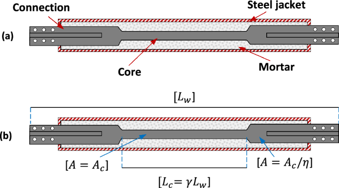
a Layout of a typical BRB, b geometry of a typical BRB

Full size image

To prevent buckling, a common issue in slender elements, the core of a BRB is encased in a metal jacket filled with mortar. This confinement allows the core to achieve compressive strength comparable to its tensile strength. Additionally, due to the Poisson effect, the core’s cross-sectional area expands under compressive loads, generating frictional resistance between the core and the surrounding mortar. As a result of these mechanisms, it is well established that the compressive strength of BRBs slightly exceeds their tensile strength. In terms of axial stiffness, this property depends on both the geometry and mechanical properties of the core material. Guerrero et al. (2016) provide the following equation to determine the axial stiffness () of these dampers:

where  is the cross-sectional area of the core, E is the modulus of elasticity of the core material,  is the total length of the BRB, and  is a shape factor determined by Tremblay et al. (2006):

The lateral stiffness  that a BRB provides to the structure where it is installed is a function of its axial stiffness and of the angle θ formed by the axis of the damper and the horizontal, i.e.:

2.2 Structural optimization

Metaheuristics are optimization algorithms that have been in use since the 1960s (Sörensen et al. 2018); however, their application in structural engineering did not emerge until the 1990s. One of the earliest examples of metaheuristics in structural design optimization was presented by Balling (1991), who applied simulated annealing to design a three-story frame building. This approach sparked considerable interest, as evidenced by subsequent studies conducted by Rajeev and Krishnamoorthy (1992), Kocer and Arora (1996), Coello et al. (1997), and Rajeev and Krishnamoorthy (1998), who optimized from single elements to complete trusses and reinforced concrete structures.

Over the years, studies on structural optimization have evolved to address the practical and standardization requirements demanded by construction processes. For instance, Hasançebi and Erbatur (2002) conducted topological optimization of trusses using simulated annealing, considering commercially available structural profiles along with their corresponding weights and dimensions. Similarly, Degertekin et al. (2008) employed genetic algorithms to minimize the weight of three-dimensional steel frames. In their approach, they not only considered commercially available profiles but also grouped structural elements to ensure homogeneity in the optimized designs.

Subsequently, more complex design conditions, such as those induced by wind (Martínez et al. 2011) or seismic excitations (Hejazi et al. 2013), were incorporated into structural optimization. Seismic optimization, in particular, is of special interest due to its computationally intensive nature and because these processes are crucial for developing more sustainable and resilient infrastructure systems (Velasco et al. 2022).

Formally, a structural optimization problem can be defined as:

Subject to:

where  and  are the constraints of the problem,  and  are the bounds of the decision variables,  is the configuration space,  is the set of feasible solutions,  is the objective function, and  is a solution formed by the vector of decision variables:

As previously mentioned, structural optimization problems can involve various objectives, such as minimizing material volumes, reducing the carbon footprint (Yeo and Potra 2015), or lowering the costs associated with the structure’s service life (Mokarram and Banan 2018). On the other hand, constraints typically involve limiting allowable stresses or deformations, depending on the specific design requirements (Velasco and Hospitaler 2021).

2.3 Artificial neural networks as surrogate models

Optimization problems involving computational simulations often require substantial time and resources. To address these challenges, researchers have increasingly turned to surrogate models, also known as metamodels, to approximate computationally expensive operations and reduce computational costs. The first study on this area introduced a framework based on Gaussian Process Regression to estimate the values of multiple objective functions, enabling the identification of promising solution candidates for direct evaluation (Jones et al. 1998). This approach optimized the resources by prioritizing high-potential solutions while avoiding unnecessary evaluations of low-quality alternatives.

Currently, surrogate models are applied in various ways to enhance optimization processes, such as facilitating the identification of promising candidates or conducting simplified feasibility assessments (Bäck et al. 2023). These applications leverage a wide range of machine learning algorithms, including Artificial Neural Networks, Random Forest, Bagging Regressors, LightGBM, and XGBoost, among others.

Artificial neural networks (ANNs) are artificial intelligence algorithms applicable in structural engineering. Thanks to their ability to predict complex behaviors with high accuracy and using a minimum of computational resources, ANNs can simplify processes such as stress determination in structural elements, structural health monitoring, or design optimization. Despite their advantages, few studies address the applicability of ANNs as surrogate models in optimizing seismic designs by metaheuristics. One of the first examples of the application of ANNs in this field was performed by Möller et al. (2009), who optimized reinforced concrete mid-rise plane frames to minimize the structure’s cost. In that study, the authors reported the feasibility of using neural networks to estimate the dynamic response of models defined by random values. The mathematical model employed by Möller et al. (2009) was defined as:

where  is the nonlinear dynamic response of the candidate solution design represented by the vector of decision variables ,  is the neural network estimate,  is the activation function, ,  are constant weights,  and  are the number of neurons in the input layer and the hidden layer, respectively, and  is the weighted input of neuron . In another study, Gholizadeh (2015) used wavelet cascade-forward back-propagation neural networks as surrogate models in the optimization process of plane steel frames. In contrast to what was done by Möller et al. (2009), Gholizadeh (2015) employed a neural network to estimate the performance levels of the solution candidates from pushover analysis and following recommendations by FEMA-273 (1997). Comparing the performances shown by the algorithm and those required by an optimization algorithm without a surrogate model, Gholizadeh (2015) reported a 98.8% decrease in execution time when using ANNs.

Gholizadeh and Mohammadi (2017) employed wavelet back-propagation neural networks to optimize the resilience-based design of mid-rise plane steel frames. Similar to their previous study, the ANN estimated the result of a pushover analysis to define whether the candidate solutions met the problem’s constraints. Mergos (2022) introduced a surrogate model that integrates design of experiments (DoE) with radial basis function (RBF) interpolation. Within this framework, the optimization algorithm employs the surrogate model to identify the most promising solution candidates, which are subsequently evaluated using high-fidelity methods, such as finite element method (FEM) simulations. The proposed approach was applied to the seismic optimization of 3D reinforced concrete frames, demonstrating its reliability and effectiveness. A noteworthy aspect of Mergos’ work is the combined use of low-fidelity (surrogate model) and high-fidelity (FEM simulations) models to guide the optimization process. This complementary strategy aligns with the principles outlined in earlier studies on surrogate models (Bäck et al. 2023) but contrasts with the methodologies adopted in more recent research.

Subsequently, Noureldin et al. (2022) formulated a methodology to optimize the seismic retrofitting of low-rise frames equipped with displacement-dependent dampers. Although the proposed methodology was capable of predicting drifts, accelerations, and basal shears, it should be noted that its applicability was limited to low-rise buildings because the neural network predicted the dynamic response of equivalent SDOF oscillators rather than the actual structure. Finally, Liu et al. (2025) developed a surrogate model based on conditional generative adversarial networks (cGAN) and applied it to optimize the seismic design of steel frames equipped with viscous dampers. In this framework, the surrogate model was used to approximate the structural response of solution candidates, replacing the need for nonlinear time history analysis (NTHA). Notably, the authors reported that the optimization process was entirely driven by the surrogate model, eliminating the use of high-fidelity evaluation methods.

Based on the characteristics of the reviewed works, Table 1 is provided in order to emphasize the contributions of this study. It is observed that only two studies have sought to predict the response of structures with seismic protection systems through neural networks (Noureldin et al. 2022; Liu et al. 2025). On the other hand, an additional uncommon feature is the combined use of high- and low-fidelity models to guide the optimization process (Mergos 2022). Finally, it is pointed out that few studies are reporting the effect on the performance metrics of metaheuristics due to the use of ANNs. Based on the above, the contributions of this study are the following: (1) A feed-forward back-propagation ANN capable of accurately predicting the response of mid-rise BRB frames subject to NTHA is developed; (2) the affectation produced by the use of ANNs in optimization algorithms is studied based on the quality of the solutions found and the execution time; (3) evidence is provided of the inability to perform optimization processes driven solely by ANNs as surrogate models; and (4) the characteristics that provide high quality to the optimized designs of the considered case study are identified.

3.1 Benchmark building

For this study, the optimization of the seismic retrofitting of a six-story, three-bay reinforced concrete 2D frame, by installing BRBs, was chosen as a benchmarking problem. It is important to mention that the benchmark problem considered in this study was chosen due to the strongly nonlinear behavior of structures equipped with BRBs, which results in computationally expensive design processes. Consequently, the metaheuristic optimization of such structures can greatly benefit from the use of surrogate models. Additionally, it should be noted that the benchmark problem was not taken from previous publications. The structure was an office building located in the soft soil zone of Mexico City and it was designed based on the 2004 version of the Complementary Technical Standards of Mexico City (2004). A layout of the structure is shown in Fig. 2, together with the dimensions of the cross sections of the structural elements.

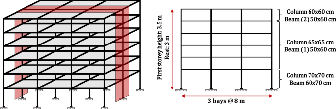
Frame studied

Full size image

The longitudinal (, ) and transverse () reinforcement ratios used in the elements are shown in Table 2. In the highest shear zones of the elements, a transverse reinforcement composed of two 3/8′′ stirrups and a 7.5 cm spacing was considered. Also, the contribution of a 20 cm slab was considered in the lateral resistance of the frame. A compressive strength of f′c = 30 MPa was considered for the concrete elements, while the reinforcing steel had a yield stress of f_y = 420 MPa. The core of the dampers was made up of steel with a yield stress of f_y,BRB = 350 MPa.

3.2 Constraints

In this study, the limit values of deformations associated with a life safety performance level, according to NTC-2023 (2023) and ASCE 41/17 (2017), were taken as constraints. Defining the maximum plastic rotation angle of the beam and column elements as θ_j^lim and the maximum inter-story drift ratio as IDR^lim, the constraint functions of the problem are as follows:

where IDR_i is the inter-story drift ratio of story i and θ_j is the plastic rotation of element j. In accordance with the provisions of NTC-2023 (2023) and ASCE 41/17 (2017), the IDR limit value was set to IDR^lim = 2%. According to ASCE 41/17 (2017), the values of the maximum plastic rotation angle should be determined as a function of the reinforcement of the elements, their level of confinement, and their level of demand. Based on the above, the θ_j^lim values can be found in Table 3.

3.3 Objective function

The algorithms were designed to minimize the amount of material used in the BRBs. As Mahrenholtz (2014) indicated, BRBs can be installed in reinforced concrete frames either by steel connections fixed through anchors or by metallic substructures. Considering the former approach and the geometric relationships of the BRBs (see Fig. 1), the objective function of the optimization problem is:

where  is the vector that defines the design, W_sd is the damper’s core weight, γ_s = 7860 kg/m³ is the specific mass of steel, L_w is the total length of the damper while A_ci, γ_i, and η_i are the core’s cross-sectional area, the length ratio, and the area ratio of the i-th BRB employed in the solution, respectively.

3.4 Decision variables and parameters

The decision variables of the problem were the location of the dampers, their cross-sectional area (A_ci), and their ratios of areas and lengths ( and , respectively). All decision variables were comprised of discrete values which are shown in Table 4. Despite the existence of BRBs of standardized measurements, manufacturers can produce these elements with any dimension required by their customers, making discretization of the decision variables possible. A ternary system was used to define the BRB arrangement, where 0 represented the absence of the damper, while 1 and 2 represented a simple-diagonal damper oriented to the right or left, respectively. It is important to highlight that an integer codification was employed in this study, as this approach ensures, in a straightforward manner, that the obtained solutions consist of decision variables with standardized values required by the construction industry. Additionally, the dimensions and reinforcement of the structural elements were taken as parameters of the problem as well as the characteristics of the materials used in the main structure and the BRBs. To avoid obtaining designs with little redundancy, it was imposed as a condition that the BRB distributions were symmetrical in terms of their location and the characteristics of their cores. Under these considerations, the size of the problem solution space, denoted as ||, is:

where k is the number of decision variables, c_i is the cardinality of decision variable i, and r is the dimension of the vector defining a possible solution to the problem. Given the conditions of the problem, and considering arrays of r = 12 elements, ||= 1.94 × 10⁴⁶ possible solutions.

3.5 Seismic demand

The feasibility of the designs generated by the algorithms was determined by nonlinear time history analysis (NTHA) using twelve synthetic acceleration records. Since the structure was considered to be located in Mexico City, the used records were those generated by SASID (2023), which were scaled so that the mean of their ordinates was equivalent to those of the corresponding uniform hazard spectrum (UHS). It is significant to mention that two main sources affect Mexico City, namely: the subduction zone and the intraslab zone. As a consequence, two types of earthquake ground motions must be considered for design purposes, i.e.: subduction (SUB) and intraplate (IP) ground motions. Both types of earthquakes were considered in the NTHA of the generated designs, with eight being subduction earthquakes and four being intraplate earthquakes. Figure 3 shows the result of the scaling of the records, where the pseudo-acceleration spectra are shown in gray, the uniform hazard spectrum in red, and the mean of the subduction and intraplate earthquake ground motions in green and blue, respectively. It is important to note that the acceleration records were obtained for the following geographic coordinates (latitude: 19.468, longitude: − 99.099), a location that corresponds to a soft soil site.

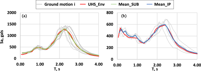
Spectra of a subduction, b intraplate

Full size image

3.6 Structural model

The OpenSeesPy library, which allows to use OpenSEES (PEER 2006) in conjunction with Python code, was employed to model and analyze the proposed designs during optimization. The element’s concrete was modeled using the Concrete02 material, considering the model of Mander et al. (1989) to define the properties of the confined concrete. For the reinforcing steel bars, the ReinforcingSteel material was used in conjunction with the MinMax material to define the ultimate deformations of the steel. Also, the reinforced concrete elements were modeled with the forceBeamColumn element using the HingeRadau method (Scott and Fenves 2006) as the integration method. Following the recommendations of Scott and Ryan (2013), the length of the plastic hinges of the elements was set equal to 1/6 of the total length. Figure 4 shows the layout of the fiber sections, as well as the monotonic and cyclic behavior of the materials that compose them. In the structural models, BRBs consisted of elements composed of fibers connected in series, representing the connections and the damper’s core (Velasco and Guerrero 2020). The axial response of the core fibers was modeled by the SteelMPF material which represents the model proposed by Menegotto and Pinto (1973) and extended by Filippou et al. (1983) to consider the effects of isotropic strain hardening.

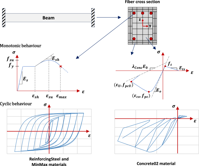
Fiber cross section and materials used in the numerical model

Full size image

Collected data during an experimental test of a full-scale BRB (Guerrero 2023) were used to calibrate the material behavior. The material’s compressive strength was defined as 15% higher than the tensile strength. On the other hand, the strain hardening ratio, in tension and compression, was set equal to 0.006 and 0.015, respectively. Through the calibration process, the remaining parameters that define the transition between the elastic and inelastic response of the material were defined (R_o = 16.0; cR₁ = 0.89; cR₂ = 0.16; a₁ = 0.015; a₂ = 6.0; a₃ = 0.03; and a₄ = 5.0). Additionally, the fatigue material was used to consider the accumulated damage in the damper core, which considers the effects of low cycle fatigue (Ballio and Castiglioni 1995) by means of Miner’s rule (Miner 1945).

A comparison between the recorded behavior in the experimental test (Guerrero 2023) and the numerical model is shown in Fig. 5a. As can be seen, both curves are quite similar. On the other hand, Fig. 5b and c presents the numerical response of the damper for length ratios = 0.25 and = 0.80, respectively. It can be seen that the calibrated model reflects the higher axial stiffness and higher post-yielding stiffness that characterizes the behavior of short-core BRBs (Mirtaheri et al. 2011; Hoveidae et al. 2015). Representing these effects is essential as they can significantly influence the characteristics of optimized designs.

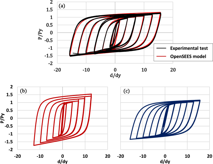
BRB material calibration; a comparison between experimental test and numerical model, b short-core BRB behavior (= 0.25), c long-core BRB behavior (= 0.80)

Full size image

3.7 Seismic performance of bare frame

The seismic performance of the bare frame was determined by NTHA and considering the twelve acceleration records provided by SASID. Figure 6 shows the IDR profile of the bare frame together with a vertical line representing the limiting IDR value. It is important to note that the IDR profile was elaborated with the average of the maximum IDRs presented by the model for each acceleration record. It is observed that the structure develops IDR with values of 4% in the second and third levels. These values are greater than the 2% established as the limit, which implies an inadequate seismic performance and justifies the retrofitting process. The highest plastic rotation of the beams presented a value of 0.014, which is below the value established as the limit; therefore, it is considered that the restrictions associated with the plastic rotations are fulfilled for the bare frame.

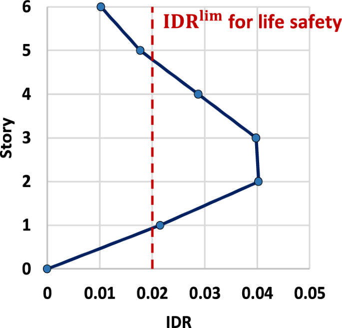
IDR profile of the bare frame

Full size image

Simulated annealing (SA) and genetic algorithms (GA) were used to solve the optimization problem. In order to study the benefits and drawbacks of using surrogate models in the optimization process, three different versions of GA and SA were proposed. In the first one, only ANNs were used to evaluate the feasibility of the designs; these versions were named GA-ANN and SA-ANN. The second version of the algorithms corresponds to a classical approach to the problem where nonlinear dynamic analysis is used to evaluate the possible solutions; these versions were named GA-NTHA and SA-NTHA. Finally, the third version uses a hybrid approach combining ANN and NTHA to explore the solution space; these versions are denoted as GA-HIB and SA-HIB. All versions of the SA and GA algorithms were self-implemented in Python. Additionally, the ANN was developed using the Keras library (Chollet 2015) in Python.

The optimization process in the GA-HIB and SA-HIB algorithms was divided into two stages: the first one, where the feasibility of the designs is verified by the ANN, and the second one, where NTHA is used. The change between both feasibility verification processes was controlled through the objective function value of the design to be reviewed. If the proposed design presented a cost above a threshold value W_lower, the feasibility check was performed by the neural network; otherwise, NTHA was used. The details of each algorithm as well as the ANN developed are given below.

4.1 Surrogate model

A sample of data from 600 different models of the studied frame was created to train the neural network. The characteristics of the dissipative system of the 600 models were randomly defined, and each design proposal was analyzed under five different acceleration records from the set of twelve synthetic accelerograms provided by SASID (2023). The five ground motions were chosen randomly and were different for each created model. A dataset of 3000 NTHA was obtained by this process, and it contained the following data: peak ground acceleration (PGA), peak ground velocity (PGV), peak ground displacement (PGD), Arias intensity and significant duration of the earthquake used, the frame’s fundamental period, the amount of material used (), and the lateral stiffness provided by the dissipative system at each frame’s level. With the input data, the ANN predicted the value of the IDR of each level of the proposed design. It is noteworthy that the generation of this sample required a computation time of 4.96 days on a computer equipped with a Xeon® E-2146G (3.5 GHz) processor and 16 GB of RAM. On average, each NTHA took 2.4 min to execute. Consequently, assessing the feasibility of a single design would take approximately 28.8 min when all twelve synthetic records are considered.

To mitigate overfitting, the dataset was split into a training set and a validation set, with the latter used to assess the network’s predictive capability. The training set comprised 70% of the data, while the remaining 30% was allocated to the validation set. The objective function values of the designs that make up the dataset are shown graphically in Fig. 7. From the data, it was found that the average design of the set uses 12,000 kg of steel in its dissipative system. Additionally, the maximum and minimum values of the sample objective function were equal to 26,749 and 2161 kg of steel, respectively.

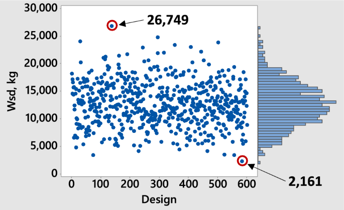
Training set data

Full size image

Neural networks consist of different types of layers, namely input, hidden, and output layers, which are typically densely connected. The neurons in these networks transmit information processed by activation functions, whose nonlinear behavior enables the learning of complex patterns from data (Mercioni and Holban 2023). As a result, the proper selection of activation functions is crucial for the effective performance of neural networks. Common examples of activation functions include ReLU, ReLU6, Softmax, Sigmoid, and Tanh, among others. ReLU and ReLU6 are quite similar, with the latter introducing an upper bound of six, which addresses the issue of the original ReLU function’s unbounded output. ReLU6 is formally defined as:

Conversely, the Softmax function is primarily used as an activation function in classification problems. It produces output values ranging between zero and one and is defined as:

where  and  are the i-th and j-th values of the input vector z. Another activation function widely used in neural networks is the Sigmoid function, defined as:

Additionally, the hyperbolic tangent function (Tanh) has output values bounded between -1 and 1, inclusive and is defined as:

In the following sections, the process of calibrating the neural network’s hyperparameters will be discussed and the impact of activation functions on its performance.

4.2 Simulated annealing

Simulated annealing (SA) is a metaheuristic presented by Kirkpatrick et al. (1983). This algorithm makes an analogy with a metallurgical industry process called annealing, in which a melt is cooled in a controlled manner to reach ordered states of minimum energy. SA uses a probability distribution as acceptance criteria that allow it to accept better solutions than the current ones and worse or degraded ones. This distribution is based on the Boltzmann distribution:

where ΔE is the energy increment, k_b is the Boltzmann constant, T is the process temperature, Z is the partition function, and P(E_n) is the probability of finding a random particle in an energy state E_n. In an optimization process, the Boltzmann constant and the partition function become unnecessary, and their values are taken equal to one. Keeping the concept of temperature, the transition probability between the current solution  and the new design found  is:

ΔE = f() – f() is the degradation of the objective function. From Eq. 16, it is observed that the probability of transition from solution  to solution  is inversely proportional to the increase of the objective function and decreases with the temperature T. Accepting degraded solutions allows the algorithm to escape from local optima; for this reason, the user needs to calibrate the initial value of the temperature as well as to choose an adequate cooling program. In practice, the most usual is to use a geometric cooling program, in which the temperature of state t + 1 is proportional to the temperature of state t using a cooling coefficient K < 1:

In SA, for each state  of temperature, a certain number of possible solutions are checked; this process results in a trajectory in which the successor state is chosen depending only on the current state (Blum and Roli 2003), which allows to define it as a Markov chain. On the other hand, the freezing criterion is used as a stopping rule, in which the search process ends when the temperature decreases to a certain percentage of the initial temperature, usually 1% or 2% of the initial temperature (Medina 2001). The SA hyperparameters used in this study are listed in Table 5. It is worth noting that, through a sensitivity analysis, it was determined that the algorithm reached its best performance when W_lower = 2300 kg.

4.3 Genetic algorithms

Genetic algorithm (GA) is a metaheuristic developed by Holland (1975) and was one of the first algorithms of this class. GA is a population-based optimization algorithm that employs the concept of natural selection to generate high-quality solutions. GA uses three basic operators to simulate the evolutionary process through natural selection: selection, crossover, and mutation (Goldberg 1989).

In GA, each solution of the population is called an individual, which is chosen to generate new solutions through a stochastic selection operator that shows a preference for high-quality individuals. Among the most commonly used algorithms as selection operators are roulette selection and tournament selection; however, it is known that, in the former, low-quality solutions may have a high probability of being selected (Blickle and Thiele 1996).

After selecting the individuals, their characteristics are combined to generate new solutions. In GA, various operators can be used for this purpose, such as one-point, two-point, or multi-point crossover (Hussain et al. 2018). The newly generated solutions are then subjected to a certain probability of mutation, where some of their characteristics are randomly modified. This last operator has two critical functions: to protect the algorithm from irrecoverable losses of valuable features and to allow the exploration of large areas of the solution space (Goldberg 1989). Finally, the new population generated replaces the old one, and the process is repeated for a given number of iterations.

In this study, GA used a tournament selection and two-point crossover algorithm. Since a low feasibility rate was observed in the designs generated, it was decided to only accept solutions in the population, i.e., GA discarded infeasible designs. It is important to note that this decision allowed better performance by generating higher-quality populations. To reduce the algorithm’s execution time, each newly generated design was compared with the existing individuals in the population to identify the potential duplicates. If a duplicate was detected, its evaluation was omitted, but the design was still integrated into the population. Conversely, if the design was unique, it was evaluated to determine whether it satisfied the problem’s constraints. Additionally, it was identified that the algorithm achieved adequate performance when W_lower = 3000 kg. The remaining hyperparameters of the algorithm are listed in Table 6.

In addition, the hyperparameter values shown in Tables 5 and 6 were applied to all three versions of GA and SA. These hyperparameters were selected to ensure similar average runtimes when using NTHA, while maintaining high-quality solutions. To define the values of the SA and GA hyperparameters, a target mean execution time was initially defined with the objective of balancing adequate exploration of the configuration space with practical feasibility. This criterion was employed because excessively long runtimes are a major limitation of metaheuristics in professional practice (Xiao et al. 2022). For the studied problem, an average runtime of 3–4 days was deemed appropriate. Based on this target, various combinations of hyperparameters were tested and iteratively adjusted until the desired performance levels were achieved. As shown in Fig. 10, this procedure resulted in very similar average runtimes for GA-NTHA (4.1 days) and SA-NTHA (3.7 days).

5.1 Artificial neural network fitting

In the training process of the ANN, the mean square error function was used as a loss function, and 150 epochs were performed. On the other hand, the input data were normalized prior to training the neural network. Seventy percent of the collected dataset was used to train the neural network, while the remaining 30% was used for the validation phase.

The Adamax algorithm was used as the optimization algorithm in compiling. Adamax is a variant of Adam algorithm which is a first-order gradient-based optimization algorithm (Kingma and Ba 2015). With the Adamax algorithm, the parameters θ of the neural network are updated by estimating the first- and second-order gradients (m_t and v_t, respectively) of a noisy objective function f(θ) for timestep t. The parameters are updated according to the following expression:

where ε is a small-valued term that avoids division by zero, and α_t is the learning rate:

being β₁ and β₂ parameters that control the decay rate. The R-squared value (R²) and the mean absolute error (MAE) were taken as metrics for the ANN fit. The R-squared coefficient was determined as:

where n is the number of observations, y_i is the value of the dependent variable, μ is the mean of the dependent variable, and ŷ_i is the value predicted by the neural network. On the other hand, the MAE is calculated as follows:

The neural network calibration process involved testing various combinations of the number of hidden layers, the number of neurons per layer, and the activation function employed. During this phase, the ReLU activation function was applied to all neurons. Each time the neural network was trained, and the sets were randomly generated to ensure data representativeness and prevent overreliance on any particular partition. The performance of each hyperparameter combination was evaluated using the coefficient of determination  as defined by Eq. (20). Table 7 displays the network fits based on the number of hidden layers and neurons considered.

It is evident that the number of neurons and hidden layers significantly influences the network fit. For instance, with 4 hidden layers and 50 neurons per layer, the network achieved a coefficient of determination . In contrast, increasing the parameters to 10 hidden layers and 200 neurons resulted in an  value of 0.94. Additionally, it is noteworthy that the increase in  values does not continue indefinitely, as similar values are obtained with 200 neurons across both 8 and 10 hidden layers. Based on these findings, further tests were conducted on the network configured with 8 hidden layers and 200 neurons per layer, utilizing different activation functions.

Table 8 presents the coefficients of determination obtained by incorporating the activation functions Sigmoid, ReLU6, Tanh, and a combination of ReLU with Softmax in the neural network. It is evident that the choice of activation function significantly influences the network’s fit. The lowest performance was recorded with the Sigmoid function, which yielded an  value of 0.07, while the Tanh function achieved . In contrast, the ReLU6 function showed no improvement in fit compared to the standard ReLU function. Notably, the combination of ReLU and Softmax resulted in a slight enhancement in fit, raising the  value to 0.96.

Based on these findings, this study opted for a neural network architecture comprising 8 hidden layers, each with 200 neurons. The first seven hidden layers employed the ReLU activation function, while the final layer utilized the Softmax function. With these hyperparameters, the ANN achieved an  value of 0.958 and a mean absolute error (MAE) of 0.0005 during the validation process. The neural network fit is illustrated graphically in Fig. 8. The predicted IDRs closely resemble those obtained through “exact” procedures, in this case, by NTHA. Furthermore, the MAE indicates a negligible mean difference between the predicted and actual values, amounting to only about 2.5% of the IDR limit value.

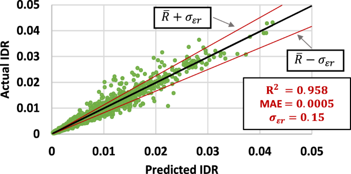
Fitting of the trained neural network

Full size image

The standard deviation of the relative error () provides a measure of the dispersion between the actual IDR values and those predicted by the neural network (Möller et al. 2009). This dispersion metric is calculated from the IDR values obtained by the NTHA () and those predicted by the network (), according to Eq. (22).

5.2 GA-ANN and SA-ANN results

Due to their stochastic nature, metaheuristic algorithms yield different solutions in each run, and the proximity of these solutions to the global optimum is neither constant nor determinable with certainty. Consequently, multiple runs are required to ensure that the algorithm consistently produces high-quality solutions. In accordance with the recommendations of Paya-Zaforteza et al. (2010) on the above point, the results presented for each algorithm in this study were obtained from 12 runs using the same hyperparameter values.

Initially, the performance of GA and SA driven solely by the neural network was analyzed. These versions were referred to as GA-ANN and SA-ANN, respectively. The average design costs obtained were 2813 kg for GA-ANN and 1952 kg for SA-ANN. Additionally, GA-ANN and SA-ANN required, respectively, 15 and 10 min on average to complete each run, thus presenting an extremely short run time. To verify that all the designs obtained met the problem’s constraints, each solution was evaluated by NTHA. A comparison between the IDR profiles obtained by ANN and NTHA is presented in Fig. 9. As can be seen, in both metaheuristics, ANN predicted lower IDR values than those obtained by NTHA. Due to this difference between predicted and actual IDR values, many of the optimized designs were not actual solutions. In the case of GA, 4 out of the 12 designs did not meet the limiting value of , while for SA this happened in 5 designs.

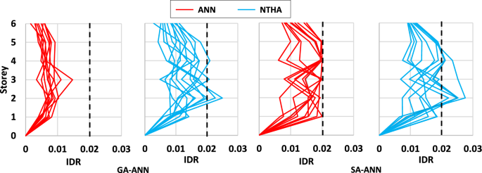
IDR profiles obtained by ANN and NTHA

Full size image

Therefore, although the ANN showed high fit metrics, it generated a considerable number of infeasible designs. In addition, as will be shown below, the designs that were feasible were of relatively low quality. The reasons behind the discrepancies between the responses predicted by ANN and those obtained by NTHA will be addressed later in the discussion section.

5.3 Optimization through NTHA and neural networks

To enhance the optimization process, this study proposes the use of ensemble ANNs and NTHAs. ANNs are employed to evaluate designs located in low-quality regions of the configuration space, while NTHAs are used to verify the feasibility of high-quality designs. This complementary strategy leverages the strengths of both low- and high-fidelity evaluations, addressing the observed limitations of surrogate models in exactly predicting the responses of high-fidelity evaluations (Liu et al. 2025). The implications of discrepancies between low- and high-fidelity assessments on the optimization process are discussed in detail in the Discussion section. To determine whether to use ANNs or NTHAs for a given evaluation, the objective function value of the candidate design is considered. Since the problem involves minimization, ANNs are applied when the objective function value exceeds a predefined threshold W_lower; otherwise, NTHAs are used. It is important to note that, in this problem, evaluating the objective function , presented in Eq. (9), is a straightforward process since it only involves quantifying the amount of the material used in the dissipative system. As a result, selecting the method to verify the feasibility of candidate solutions does not require significant computational time.

For simplicity, the algorithms that used the approach of alternating evaluations by ANNs and NTHA were denoted as GA-HIB and SA-HIB, while SA-NTHA and GA-NTHA denote the versions that only use NTHA throughout the optimization process. Each algorithm was run twelve times. For each run, the trajectory of the algorithm, the execution time, and the characteristics of the best solution were recorded.

For GA-HIB and SA-HIB, threshold values of 3000 kg and 2300 kg of steel were established. These values were determined based on the results obtained from GA-ANN and SA-ANN, where both algorithms were observed to generate infeasible designs for costs close to 2800 kg and 1900 kg of steel, respectively. A reduced set of performance tests with threshold values near 2800 kg for GA-HIB and 1900 kg for SA-HIB confirmed that the values that effectively prevented the classification of infeasible designs as solutions were 3000 kg for GA-HIB and 2300 kg for SA-HIB.

Figure 10a shows the boxplot of the dissipative system costs of the twelve solutions found by each algorithm. It can be observed that the two algorithms with surrogate model showed a differentiated performance compared to their versions with NTHA. For the case of GA, the average cost of the solutions found by the NTHA version was 2903 kg of steel, while for its version with the surrogate model, the average cost was 1730 kg. About SA, the solutions found by the NTHA version showed an average cost of 2065 kg, decreasing this value to 1010 kg for the version with ANN. These values indicate a decrease in the average cost of the solutions by 40% and 51% when using surrogate models. Another noteworthy feature is the decrease in the dispersion of solution costs when using ANNs. The algorithm with the lowest dispersion was SA-HIB, which presented a standard deviation of 140 kg. This dispersion value was 78% lower than that of SA-NTHA, which reached a standard deviation of 627 kg.

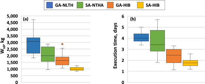
Boxplots of a solution costs, b execution times

Full size image

Figure 10b shows the boxplot of the execution times required by the studied algorithms. Similar to what was observed for the solutions’ quality, a differentiated performance is observed among the search algorithms. For this performance metric, the mean execution time for GA-NTHA and GA-HIB was 4.1 and 2.3 days, respectively. Concerning SA-NTHA and SA-HIB, the mean execution times were 3.7 and 1.8 days, respectively. These changes in run times represented a 43% and 51% decrease when using ANNs in the optimization process. Again, SA-HIB presented the smallest dispersion in execution time, showing a standard deviation of 0.4 days. The standard deviations for GA-NTHA, SA-NTHA, and GA-HIB were 0.46, 1.20, and 0.73 days, respectively.

The number of actual evaluations (NTHAs) performed by each algorithm was recorded. On average, GA-NTHA and SA-NTHA completed 2952 and 2664 evaluations, respectively. In contrast, GA-HIB and SA-HIB averaged 1584 and 1368 evaluations, demonstrating that the use of surrogate models effectively halved the number of NTHAs in both cases. On the other hand, it is important to consider that the analyses required for the development of the neural network also demanded a certain amount of time and computational resources. Therefore, for a fair comparison in terms of solution quality, it would be needed to compare the GA/SA-HIB with GA/SA-NTHA optimization processes with equivalent total number of high-fidelity (here NTHA) evaluations (e.g., to set the stopping criterion of GA/SA-NTHA optimization processes up to 3000 + 1584/3000 + 1368 evaluations, respectively) in the experimental results. However, it is important to note that the greater the number of uses given to the neural network, the shorter the execution time added to the optimization process.

Figure 11 shows the trajectories followed by the four algorithms in their twelve runs. The trajectories of each algorithm that achieved the highest quality solutions and those that required the shortest execution time are shown in color. From the figures, it is observed that SA-NTHA presented prolonged decreases in the value of its objective function, requiring several hours to reach solutions with costs less than or equal to 5000 kg of steel. Another relevant observation is the steep drop in SA-HIB and GA-HIB trajectories, which show that the algorithm achieved solutions with costs of less than 3000 kg of steel in fractions of an hour. This rapid decrease in the value of the objective function in ANN algorithms was because it was computationally less expensive to verify the feasibility of designs using ANN than NTHA. Due to this feature, algorithms with surrogate models could quickly abandon low-quality regions and use the time saved to explore areas with high-quality solutions further.

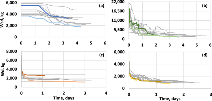
Trajectories followed by a GA-NTHA; b SA-NTHA; c GA-HIB and d SA-HIB

Full size image

The review of the considered constraints in the optimization problem revealed that the IDR were the response that most conditioned the proposed designs; for this reason, these are described in greater detail. The IDR profiles developed by the best solutions achieved in each algorithm run are shown in Fig. 12. It is worth mentioning that the IDR profiles were obtained by NTHA and were constructed with the average of the maximum drifts developed by each of the 12 synthetic acceleration records. Since a limit value of 2% was considered, the graphs use this value as the maximum on their horizontal axes. Likewise, the solutions of each algorithm with higher qualities and lower execution time are distinguishable due to the use of colored lines that follow the same color code used in Fig. 11.

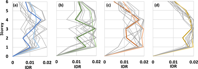
IDR profiles of the solutions found by a GA-NTHA; b SA-NTHA; c GA-HIB and d SA-HIB

Full size image

The IDR profiles show the degree of optimization of the solutions achieved by the search algorithms. It can be seen that the solutions found by GA-NTHA presented an IDR profile far from the limit value, which denotes that these solutions are conservative designs that do not efficiently use the material of their dissipative system. On the other hand, the solutions found by SA-HIB showed a response very close to the limiting IDR value, which corresponds to the high quality of the solutions found by the algorithm. Given the degree of similarity between the limit value and the IDR profiles of the solutions found by SA-HIB, it can be said that the global optimum of the problem presents a material cost close to the average cost of the solutions found by this algorithm.

5.4 Analysis of optimal solutions

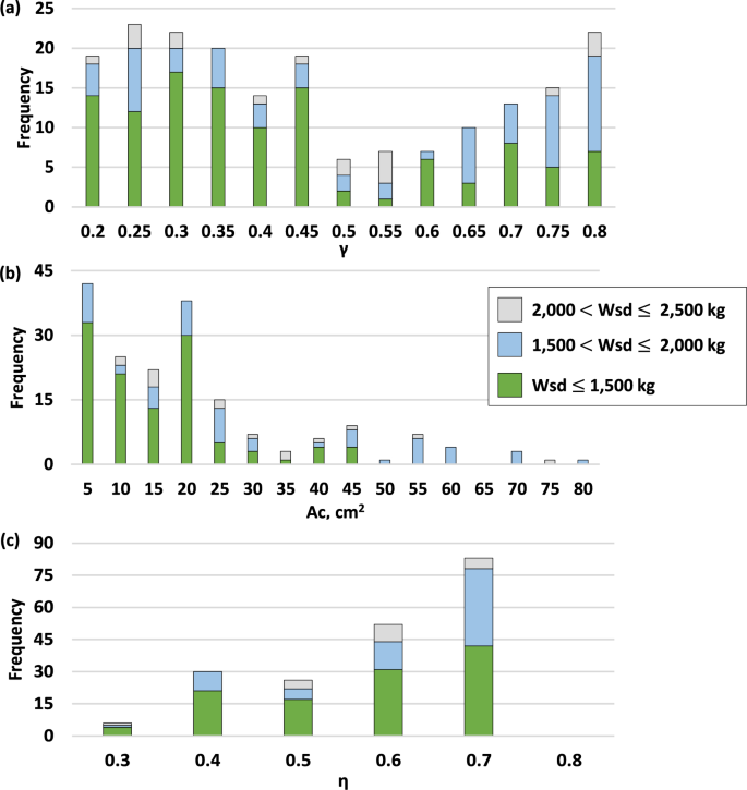
The 12 runs of GA-NTHA, SA-NTHA, GA-HIB, and SA-HIB produced 48 optimized solutions, which were further studied to identify the characteristics that allow them to show high seismic performance. Figure 13 shows the frequencies of the different values that constitute the decision variables of the problem, i.e., the length ratio (), the cross-sectional area of the damper core (), and the area ratio (). Additionally, the characteristics of the decision variables were grouped according to the value of their objective function. To facilitate the interpretation of Fig. 13b, only the frequencies of the values  80  are provided; however, that interval includes 95% of the data obtained for that decision variable.

Frequencies of values used for a length ratio ; b cross-sectional areas; and c) area ratio 

Full size image

For the  ratio (Fig. 13a), a high frequency of values 0.8, 0.45, and between the range of 0.2–0.35 is observed; however, if only those solutions with costs  kg are considered, a great preference of the algorithm for values  is observed. On the other hand, the optimized designs mainly used values of  between 5 and 20 , with values greater than 50  only being observed in designs with costs greater than 1500 kg. Finally, for the  ratio, values between 0.4 and 0.7 were mainly used.

From Fig. 10a, it can be seen that GA-NTHA and SA-HIB were the algorithms that presented the worst and best performance. To better understand the variation of solution characteristics as a function of their quality, Fig. 14 shows the four worst solutions of GA-NTHA. In comparison, Fig. 15 shows the four best solutions obtained by SA-HIB. About the GA-NTHA solutions, the lowest quality designs used 12 to 6 dampers, slightly contrasting to the SA-HIB solutions, which used 8 to 5 dampers. Other significant differences were found in the distribution and cross-sectional area of the BRBs. In the solutions found by SA-HIB, the suppression of the BRBs is observed in the first, fifth, and sixth levels. Recalling the IDR profile of the bare frame (see Fig. 6), it is observed that no dampers were used in those levels with the lowest IDR magnitudes. On the other hand, in the highest quality solutions, BRBs with cross-sectional areas of up to 25 cm² were used, which contrasts with the use of dampers with dimensions of up to 100 cm² in the designs obtained by GA-NTHA.

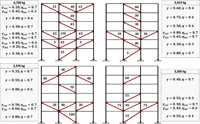
Solutions found by GA-NTHA

Full size image

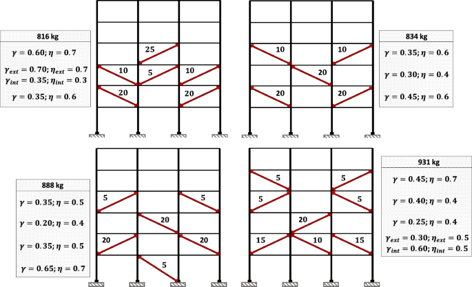
Solutions found by SA-HIB

Full size image

The objective of this study was to identify the effects of using ANNs as surrogate models in the metaheuristic optimization process. In order to achieve this objective, this study was based on the theory that every metaheuristic is an algorithm made up of different components that play a specific role in its performance (Johnson et al. 1989; Sörensen 2013; Franzin and Stützle 2019). As ANN is considered as the component to be studied, the performance of the classical versions of SA and GA is only compared with that of their ANN versions. Additionally, other algorithms are not considered since their performance metrics would only provide helpful information for this study if they were compared to their respective surrogate model versions. In that sense, this paper should not be confused with other studies that only seek to demonstrate the high performance of a new metaheuristic and that have been so harshly criticized recently (Aranha et al. 2021; Tzanetos and Dounias 2021; Kudela 2022).

Although other studies have been published where seismic designs are optimized with the help of ANNs, these works have not investigated the limitations and effects of these surrogate models on the performance of the optimization algorithms. Through the tests performed in this research, it was identified that surrogate model cannot satisfactorily drive the whole optimization process. As shown in Fig. 8, if an optimization algorithm relies solely on a surrogate model, such as ANNs, it will likely return a design that fails to meet the problem’s constraints; this situation occurs even though the surrogate model exhibits high fit metrics. The reason for this problem is considered to lie in the characteristics of the training set, which is explained with the help of Fig. 16.

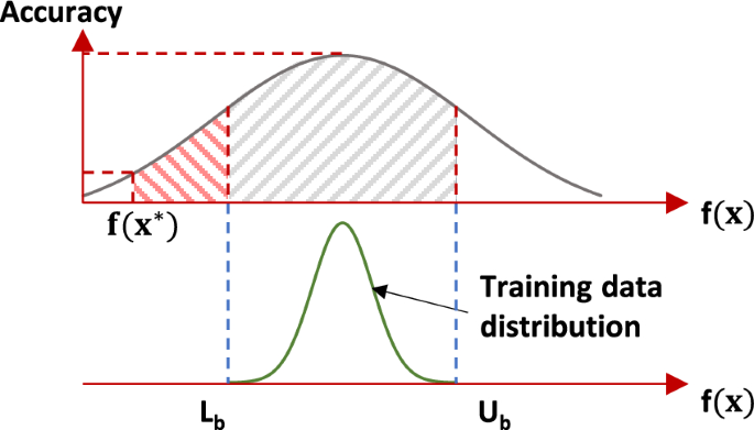
Accuracy of the surrogate model as a function of design quality

Full size image

Figure 16 schematically shows the accuracy of a machine learning surrogate model, such as an ANN, as a function of the value of the objective function of an optimization problem and its relationship with the training set used. The training set will generally present a frequency distribution bounded in a lower by  and in an upper by . Considering a minimization problem and given the random process through which the training set is generated, the value of the global optimum objective function, denoted here as , can be expected to be considerably less than the lower bound  of the training set. For example, in this study, the value of  was 264% larger than the value of the highest quality solution found.

The discrepancies between the characteristics of a randomly generated design and those of the global optimum are of vital importance because the predictive capability of a machine learning algorithm depends on the information present in its training set. If the algorithm seeks to predict the response of a system similar to those found during the training process, it is expected to provide a good prediction. For these reasons, and as shown in Fig. 16, the accuracy of the surrogate model reaches its maximum in the region of maximum frequency of the training set distribution. However, this level of accuracy is not constant and decreases for designs outside or near the extremes of the training set distribution. Given that there is only a single global optimum for any given optimization problem, it is unlikely that a machine learning algorithm could predict the response of that solution with high accuracy.

To study the implications of discrepancies between surrogate models (low-fidelity models) and high-fidelity models (FEM simulations), a schematic representation is provided in Fig. 17. For clarity, the discussion is centered on IDR, although the underlying concepts are broadly applicable to any response estimated using surrogate models. Figure 17 depicts the IDR curves predicted by a low-fidelity model for two designs: A and B. Design A represents a suboptimal solution, while design B corresponds to a high-quality solution. Due to inherent differences between surrogate model predictions and high-fidelity simulations, uncertainty is introduced. This uncertainty is illustrated in Fig. 17 as shaded gray regions around the IDR curves, indicating the surrogate model’s potential to either underestimate or overestimate the responses generated by the high-fidelity model.

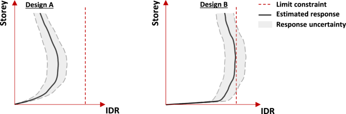
Comparison of estimated and actual responses for low- and high-quality designs

Full size image

For design A, the deviation between the estimated and actual responses does not significantly affect the optimization process. Since design A represents a low-quality solution, even a substantial underestimation of the actual response would not violate the limiting response constraint (). However, this situation changes in the later stages of the optimization process, as high-quality solutions begin to emerge. This scenario is represented by the response scheme of design B. As shown in Fig. 12d, highly optimized designs tend to exhibit responses very close to the constraint limit. In such cases, even small deviations between the estimated and actual responses can have significant implications for the algorithm’s direction, potentially leading to the misclassification of infeasible designs as viable solutions. This misclassification is highly undesirable, as it disrupts the optimization process, misguides the algorithm, and may result in erroneous conclusions about the problem under investigation.

It is important to emphasize that the scenario described above is only expected to occur when surrogate models are used to drive the entire optimization process. Unfortunately, numerous studies in the literature adopt such an approach (e.g., Möller et al. 2009; Gholizadeh 2015; Gholizadeh and Mohammadi 2017; Noureldin et al. 2022; Liu et al. 2025). Notably, early research on the use of surrogate models did not advocate for their complete substitution of high-fidelity models but rather proposed their complementary use (Jones et al. 1998). In this context, only one recent study was identified that follows this joint approach, that is, leveraging both surrogate models and high-fidelity methods to guide the optimization process (Mergos 2022).

Building on the reasoning presented above, this study utilized an ANN as a surrogate model to explore low-quality regions of the design space, that is, areas where even significant underestimation of the actual response does not compromise the optimization algorithm’s performance. Conversely, high-quality regions, where the ANN’s accuracy might diminish, were explored using NTHA. Although this strategy demonstrated effectiveness, it also has certain limitations, particularly in its need to develop a more refined criterion for transitioning between low- and high-fidelity models. Possible improvements to the joint use of low- and high-fidelity models include conducting statistical analyses to identify regions of the search space where the surrogate model may exhibit inaccuracies or incorporating high-fidelity evaluations during the optimization process to monitor and enhance the surrogate model accuracy. However, further research is needed to evaluate the advantages and limitations of these approaches.

Finally, it is mentioned that a relationship between the characteristics of the optimized designs and their quality was observed. As shown in Fig. 13, the optimized designs only begin to show a predilection for short-core BRBs once the value of their objective function drops below 1500 kg of steel. Something similar occurs for dampers with cross-sectional areas smaller than 20 . Because of this difference of the characteristics in optimized designs as a function of their quality, a surrogate model suitable for a specific quality range may not be suitable for another. Given its possible implications for designing optimization algorithms with surrogate models, further research considering trained surrogate models with higher proportions of high-quality designs is essential.

This paper studied the applicability of ANNs as surrogate models in a seismic optimization problem. The problem was to optimize the retrofitting of a medium-rise reinforced concrete frame using BRBs while adhering to performance-based seismic design guidelines. Given the limitations of this study, the following future work is recommended:

• Investigate the performance impacts of other metaheuristics when using surrogate models.
• Study the performance of metaheuristics with surrogate models when applied to optimize seismic designs of low- and high-rise BRB frames.
• Investigate more refined criteria to identify those regions of the search space where the ANN may present inadequate accuracy to further guide the optimization process.

Derived from the results, the following conclusions are offered:

• ANNs can be used to predict the nonlinear dynamic response of BRB frames; however, their development is problem-dependent and requires considerable time.
• Because high-quality solutions represent a minimum percentage of all possible designs in a seismic optimization problem, machine learning algorithms will have trouble accurately predicting their dynamic response, regardless of their fit metrics.
• Using only ANNs to drive a seismic optimization process will cause the algorithm to return low-quality solutions and, in some cases, even infeasible designs.
• To successfully perform a seismic optimization process, it is necessary to employ complementary strategies between ANNs and high-fidelity analysis, such as NTHA.
• Seismic optimization problems can benefit greatly from the use of ANNs as surrogate models. In the study case, the use of ANNs resulted in a reduction by 43–51% in execution time compared to versions of the algorithms without surrogate models.
• In the highest quality solutions found, the designs did not employ dampers in the first, fifth, and sixth levels; additionally, a high frequency of short-core BRBs (i.e., with ratios ) was observed.
• The characteristics of optimized designs can vary considerably depending on their qualities. In this case, only those solutions with costs less than 1500 kg of steel showed a predilection for using short-core BRBs.