Article Content
1 Introduction
In recent years, the application of UAVs has become widespread in most industries. Among these, quadrotors have achieved exceptional flexibility and stability in terms of flight dynamics. This allows their wide use in various critical and commercial domains, such as aerial surveillance, logistics, emergency response, entertainment, and agricultural monitoring. These applications are highly diverse and place very specific demands on the quadrotor; they require design such that speed, agility, and minimum weight are the priorities for executing tasks in navigation with very high precision. These UAVs must be resilient, following their predetermined flight paths despite constantly changing and unpredictable environmental factors, such as wind gusts and atmospheric disturbances. This combination of agility, speed, and robustness makes quadrotors an important component in modern UAV operations. Prior studies have explored MPC for UAVs, monolithic implementations often suffer from high computational costs, limiting real-world applicability.
Existing research on model predictive control (MPC) for UAVs has predominantly relied on single-layer architectures, which are hindered by substantial computational demands that restrict their practical deployment. To overcome this limitation, our work presents a novel cascaded MPC framework that decouples the control challenge into distinct translational (altitude) and rotational (attitude) subsystems. This hierarchical approach resolves the curse of dimensionality inherent in traditional MPC designs while maintaining robustness, thereby enabling efficient implementation on UAV platforms with constrained computational resources.
While this study focussed on mangrove forests, we acknowledge that similar environmental challenges, such as the variability of wind velocity and direction, are present along seashores. These factors contribute to the uncertainties in UAV measurements and warrant further investigation. Future work will expand the scope to include seashores and other coastal areas to compare the impacts of wind-related uncertainties across different ecosystems.
UAVs in windy environments may cause serious technical and operational issues, particularly in mangrove ecosystems. This wind turbulence is intricate and dynamic in the setting; it could be dangerous to the UAV stability and navigation system accuracy. Any disturbance from the environment will cause a deviation in the trajectory, which reduces stability and limits the efficacy under such conditions. Complex wind patterns, determined by dense vegetation and rugged terrain, require advanced control algorithms and navigation techniques specifically tailored to cope with these problems. A proper understanding of the aerodynamic interaction of UAVs with turbulent air in the mangrove canopy is essential to reduce wind disturbance and ensure safety and efficiency of UAV operation within this environmentally sensitive area.
However, designing flight systems that can cope with such disturbances at work or play poses numerous challenges, particularly when confronted with uncertainties in both familiar and unfamiliar environments [1]. Further, major stakes have even been raised because the chances of UAV failures are very high unless effective stabilization and recovery methods are put into place for the UAV industry, from external perturbations to payload fluctuations and sudden changes in the environment. This will contribute significantly to the development of UAV technology, as these are the greatest setbacks in the UAV field. Such problems introduce disturbances in the dynamic system and along the path of the UAV, which causes the UAV to lose track of its desired path. However, all of these issues can be resolved using advanced control techniques and algorithms. Such strategies contribute to the stability, safety, and efficiency of flight operations and facilitate the opportunity to improve resilience to a variety of disturbances in both normal and complex environments [2].
Of all the external disturbances, the most difficult problem for rotorcraft UAVs arises from wind gusts and turbulence, owing to their stochastic and nonlinear unpredictable nature. A typical example of a stochastic variable is wind gust; its fluctuation in wind speed is induced by alterations in atmospheric pressure and temperature changes [3]. There are two major approaches for representing gust wind: natural gust wind and mathematical models. Natural gust wind is usually measured using flow sensors and ultrasonic anemometers, and wind tunnels help in estimating the speed and direction of the wind. In contrast, methods such as continuous gust modelling, discrete gust modelling, and computational fluid dynamics provide simulation techniques for wind [4]. For example, continuous gust modelling simulates continuous gust variations using continuous probability distributions of wind gusts [3]. The widely applied model in this regard is the Dryden model, which acts like a pulse-shaping filter that identifies turbulence spectra using the power spectral density (PSD) function that describes how the power of a signal or time series is distributed across different frequency components. It provides a measure of the strength (power) of the variations of a signal as a function of frequency. It is mathematically defined as the Fourier transform of the autocorrelation function of the signal as follows:
where: is the power spectral density at frequency , denotes the Fourier transform, is the autocorrelation function of the signal, and is the time lag between two signal samples. In such a model, turbulent gust is postulated to be random, isotropic, and homogeneous [5].
2 Related work
Various control strategies have been developed to satisfy the demanding requirements of advanced control systems, ranging from simple techniques to highly sophisticated methods. Beyond PID control, a linear-quadratic regulator (LQR) represents a more advanced control approach. LQR is relatively straightforward to implement and can efficiently handle complex multiple-input multiple-output (MIMO) systems, making it versatile for engineers dealing with intricate control problems [6]. Another significant development is feedback linearization (FL), which employs a model inversion technique to achieve linearization. This method circumvents common linearity limitations and provides a more effective control mechanism under varying operational conditions [7]. Although these strategies provide sufficient control responses, they exhibit limitations in terms of their robustness. Many do not consistently achieve zero setpoint errors over time, and residual errors persist despite advanced designs [8, 9]. Consequently, continuous improvements in control strategies are necessary to address the emerging technological challenges.
Efforts to improve the wind resistance of quadcopters have led to significant advancements in the control algorithms [10,11,12,13,14]. Recent studies have explored variations in PID controllers augmented with reinforcement learning or optimized using genetic algorithms and simulated annealing. These approaches have demonstrated improved stability and accuracy under windy conditions through simulations [10, 12, 15]. Reinforcement learning has been shown to provide robustness up to a wind speed of 36 km/h under certain conditions [14].
Additionally, research has focussed on minimum-cost variance control for turbulence mitigation [11] and comprehensive wind field modelling for more realistic simulations [13]. However, although these studies provide promising insights, they are predominantly based on simulations with simplified wind models that lack real-world validation. Furthermore, most studies have been limited to specific wind scenarios or manoeuvring tasks, such as take-off, landing, trajectory tracking, and stability analysis, thereby restricting their general applicability.
Model predictive control is an advanced control strategy designed to manage multivariable processes. MPC employs an optimal control algorithm that prescribes inputs to minimize a predefined cost function while ensuring that the system dynamics remain within operational constraints over a given time horizon [16]. This approach is highly effective in regulating complex nonlinear systems while maintaining operational safety [17]. However, implementing MPC in real-time applications presents significant challenges, particularly in large-scale systems. Issues, such as system reliability, computational resource demands, and software complexity, pose considerable obstacles [19]. The literature critically reviews various real-time applications where MPC methodologies have been applied to address these challenges [16,17,18,19,20,21,22,23,24,25]. With ongoing advancements, the feasibility of applying MPC to quadrotor control in complex tasks continues to improve.
Recent works have demonstrated substantial progress in MPC for quadrotor control [27,28,29,30,31,32,33]. One notable contribution is a hybrid integral sliding mode and MPC approach that enhances trajectory tracking under disturbances [27]. To mitigate the computational complexity of MPC, Laguerre function-based input sequence approximation has been proposed, reducing computational effort while improving internal control [28]. A simplified optimal control problem tailored for small-scale quadrotors has also been developed using a ‘bang-bang’ MPC approach [29]. Furthermore, nonlinear MPC (NMPC) has been successfully implemented to enhance adaptability in handling complex drone operations [30].
System failures are inevitable in real-world applications. Research has explored NMPC for stabilizing quadrotors during rotor failures [31]. Additionally, quadrotors must be designed to handle modelling uncertainties, prompting the development of an adaptive NMPC that incorporates real-time learning and model adjustments. This approach has significantly improved quadrotor robustness, reducing tracking errors by 90% compared to non-adaptive NMPC with minimal computational overhead [32].
Further advancements include NMPC-based obstacle avoidance methods. One study introduced a penalty term based on potential field functions, incorporating an adaptive prediction horizon to alleviate the computational burdens [33]. Another approach utilizes algebraic ellipsoids to represent obstacles, demonstrating efficiency in navigating dense environments [34]. Despite significant progress in applying MPC to unmanned systems [35], major challenges remain, particularly in high-speed real-time applications. The complexity of MPC stems from its reliance on a fully nonlinear quadrotor model, making it computationally intensive and unsuitable for real-time control. Consequently, linear control schemes have been explored owing to their simplicity and ease of implementation [36]. Linearization techniques, including trimming at zero wind and hover conditions, enable single linear time-invariant (LTI) modelling for MPC applications [35, 37, 38].
Recent advancements have further refined MPC for quadrotor control. Li et al. [39] introduced a flatness-based MPC framework incorporating a DenseNet neural network to improve trajectory planning through inverse dynamics learning. Similarly, Hui et al. [40] developed a dual-cascade MPC integrated with H-infinity control to enhance UAV stability in turbulence. Additionally, Chen et al. [41] proposed a hybrid method combining a nonlinear extended state observer (NLESO) with sliding mode control (SMC) to enhance the real-time responsiveness in windy conditions. These approaches collectively demonstrate improvements in the UAV stability, trajectory tracking, and wind resistance.
To further improve adaptability, researchers have explored neural-network-based adaptive control. Madebo et al. [42] developed a model reference adaptive control (MRAC) framework utilizing neural networks for dynamic parameter adjustment. Zhang et al. [43] proposed a fixed-time extended disturbance observer (FTEDO) to switch between PID and ADRC based on wind speed. Similarly, Muthusamy et al. [44] introduced a fuzzy-based intelligent controller that can autonomously adapt to wind disturbances. Optimization-based strategies have garnered considerable attention. Li et al. [45] integrated MPC with neural networks to minimize tracking errors, while Bannwarth et al. [46] proposed an H-infinity controller to optimize control forces in windy conditions. Wang et al. [47] introduced an SMC-based approach with a state compensation function observer, improving tracking accuracy by 61.2%. Collectively, these studies highlight a shift towards intelligent, adaptive, and computationally efficient UAV control methodologies.
This paper is structured as follows. Section 2 provides a critical analysis of the literature review related to this topic, and Sect. 3 provides an overview of wind turbulence in mangrove ecosystems and the quadrotor UAV dynamic model. Section 4 discusses the MPC control technique and details the proposed system for the simulation, including comparisons with the PID control structure. Section 5 presents the simulation and experimental results and analyses the performance of both controllers. Finally, Sect. 6 concludes the study and outlines future research directions.
3 Mathematical model
3.1 Modelling of wind turbulence
Turbulent wind flow is characterized by continuous and unpredictable variations, with steady wind being a component of this dynamic system. The causes of turbulence depend on several factors, including the configuration of topographical features, wind shear, heat exchange, and vortices generated by other aircrafts. In a mangrove area, factors, such as dense vegetation, varying canopy heights, and the unique microclimate of the ecosystem, interact to influence the formation and behaviour of turbulence. The complex structure of mangrove forests, along with irregular wind patterns created as air moves through branches and leaves, further intensifies turbulence. Additionally, aerial roots and water channels contribute to terrain roughness, making wind flow highly unpredictable. In engineering practice, the standard approach for accurately describing and modelling atmospheric turbulence relies on the theory and methods of stochastic processes.
The Dryden model and Von Karman model are two of the most common models for turbulence. Both models rely on detailed measurements and statistical data to determine the various turbulence characteristics. The fundamental difference between the two models lies in the process of deriving turbulence functions. The Dryden model derives the spectral function after establishing the correlation function of turbulence. The Von Karman model first establishes the spectral function and then derives the correlation function of turbulence. Despite this methodological difference, research has shown that there is no significant difference in the performance of the models. The major variation lies in the slope of the high-frequency band of the spectral function. Thus, both models are suitable for solving engineering problems related to turbulence.
This work will focus on the Dryden model as the best choice because the characteristic simplicity ensures that implementation is easier, and that the computational intensity will be lower in comparison with the Von Karman model. This advantage is particularly significant in applications in which fast simulations are required with low computational resources. The Dryden model first comes in the form of a correlation function, which is then used to obtain a spectral function.
Furthermore, the spectral functions derived from the Dryden model exhibit similarities to the basic functions that satisfy the geometric boundary conditions found in recent studies on geared shaft vibration and dynamics (Chowdhury & Yedavalli [48] and Chowdhury & Yedavalli [49]. These studies highlight the importance of spectral function formulation in understanding dynamic responses under different boundary constraints, which also has implications for wind turbulence modelling in UAV applications. By recognizing these parallels, we can enhance our understanding of how spectral functions influence system stability and control performance in dynamic environments.
This model is therefore quite representative of turbulence but less accurate in the capture of detailed high-frequency turbulence when compared to other models. Notwithstanding, the Dryden model still finds its use at lower altitudes because of its practicality. The simplicity of the Dryden model in comparison with other models gives it the potential for easy incorporation into system-level simulation and analysis tools without overburdening the computational system, especially in the areas of control system design for aerospace and automobiles. For this reason, it is a go-to model for engineers working on the stability and control of aircraft, missiles, and wind turbines at low heights. In addition, the easy implementation of this model is beneficial in educational settings because students can learn and apply turbulence modelling without involving themselves in the steep learning curve that more sophisticated models require.
Cases in which the Dryden model is preferred are those in which simplicity in computation cannot be ignored. For example, during the initial stages of design, or when there is a need to perform numerous simulations within a short period of time, the computational efficiency of the Dryden model proves to be useful. Generally, although the Dryden model may not be considered the best model for high-frequency representation, its simplicity versus efficacy has proven to be very useful in most engineering and scientific applications [50]. The Dryden spectral function can be expressed as
where , , and are the spectral function of turbulent flow whose directions are along the axis of UAV body coordinate system. , , and are the constant wind speed in three directions. , , and are the characteristic wavelength of turbulent flow in three directions.
In a mangrove environment where wind turbulence is influenced by both natural and environmental factors, selecting an appropriate model involves considering the specific characteristics of the area. The models can be adapted and calibrated using local measurement data to ensure an accurate representation of the turbulent flow. This adaptability is crucial for applications, such as the design of UAVs and other engineering solutions that must operate efficiently under challenging and dynamic conditions. To better understand the nature of wind in mangrove forests, we conducted a one-month measurement of wind speed and direction in the nearest mangrove forest situated in the Kuching Wetlands National Park, as shown in Fig. 1.
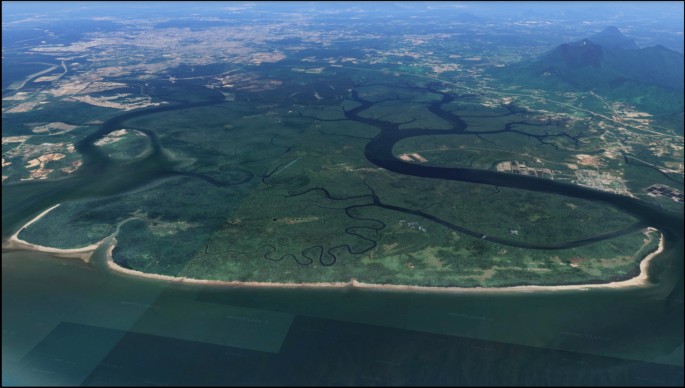
Wetlands National Park, Kuching Latitude and Longitude of the location is as follows: (Latitude: 1.6975065406193104, Longitude: 110.25447875010885)
For wind monitoring, we did not adhere to specific time intervals, as outlined in the literature, because the primary goal was to observe the overall environmental conditions in the mangrove forest. While existing studies typically suggest time intervals ranging from 5 to 10 min for measuring wind parameters, our study was designed to capture broader trends and thus did not focus on specific time intervals. This choice was made to ensure that our analysis encompassed a wide range of spatial factors. However, future studies should explore the impact of temporal resolution on UAV measurements following standard wind monitoring practices.
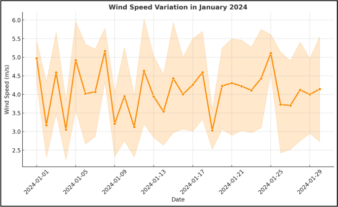
The results gotten after one-month period of measurement are shown in Figs. 2 and 3:
Recorded Wind Speed for January
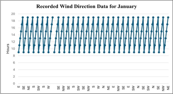
Wind direction recorded for January (Note. Recorded Wind Direction for January is from the article: Sadi, M.A., Jamali, A., Kamaruddin, A.M., & Jun, V.Y. (2024). Cascade Model Predictive Control for Enhancing UAV Quadcopter Stability and Energy Efficiency in Wind Turbulent Mangrove Forest Environment. e-Prime—Advances in Electrical Engineering, Electronics and Energy)
Figure 2 illustrates the daily fluctuations in wind speed using a line plot that includes a shaded confidence interval. The plot captured the variability in wind speed, highlighting peaks and troughs that indicate stronger and calmer wind periods. The inclusion of the confidence band provides insights into the range of expected variations, helping identify trends and extreme wind events.
Figure 3 shows the wind direction observations over different hours of the day throughout the month. The data are plotted in a pattern that highlights the periodicity of wind direction changes, showing frequent transitions among various directions, such as E (east), NW (northwest), NE (northeast), and south (S). This visualization aids in understanding wind trends and possible dominant wind directions during the month.
3.2 UAV quadcopter modelling
The Newton–Euler formalism, widely used in most previous studies, allows one to formally describe the dynamic features of the quadrotor [51]. This formalism introduces two rigid reference frames that fully describe the quadrotor movement. Here, the first one is the inertial frame ()—it is an assumed fixed reference frame, usually taken to have its x–y plane aligned with the Earth’s surface and serves as the global coordinate system. The second frame is the body frame of the quadrotor (), which is a moving reference frame that is fixed in the quadrotor’s body and rotates with it. These two frames, illustrated in Fig. 4, are critical for characterizing the position of the quadrotor relative to the inertial frame, and the orientation of the quadrotor relative to that frame. The first characterizes the position of the centre of mass of the quadrotor about the inertial frame, while the second is described by the angles of the axes of the body frame with respect to the axes of the inertial frame.
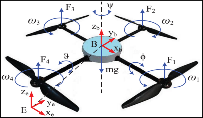
UAV Quadcopter Frame Configuration (Note. UAV Quadcopter Frame Configuration is from the article: Sadi, M.A., Jamali, A., Kamaruddin, A.M., & Jun, V.Y. (2024). Cascade Model Predictive Control for Enhancing UAV Quadcopter Stability and Energy Efficiency in Wind Turbulent Mangrove Forest Environment. e-Prime—Advances in Electrical Engineering, Electronics and Energy)
A similar approach is found in (Chowdhury & Yedavalli [50]), where the belt deflection is determined in the local belt coordinate system and the shaft equations of motion are transformed into the belt local coordinate system. This transformation approach enables the accurate representation of motion interactions between different dynamic components and is crucial for correctly modelling coupled mechanical systems. By drawing this analogy, we reinforce the importance of local–global reference frame conversions in UAV modelling, as they help capture the complex interactions between different moving components in dynamic flight conditions. By incorporating these references, we established a broader theoretical foundation for our modelling approach, linking UAV wind turbulence dynamics to well-established concepts in mechanical vibration and system dynamics.
Each propeller contributes individually to the overall movement of the quadrotor system, with the force generated by each propeller collectively contributing to the quadrotor’s thrust.
In this model, the lift constant is denoted by k and the angular velocity of the rotor by ω. Given the upward orientation of the four rotors, the resultant total thrust is aligned with the axis and is calculated as the sum of the forces generated by each individual rotor. Within an inertial reference frame, the absolute position of an object is determined by two vectors:
- Linear position vector (ξ): This vector describes the object’s position in three-dimensional space using Cartesian coordinates (, , ).
- Angular position vector (η): This vector defines the object’s orientation using Euler angles (roll—ϕ, pitch—θ, and yaw—ψ).
(7)(8)
Conversely, the body frame is characterized by a linear position vector, denoted as σ, which specifies the location of the object’s centre of mass within this frame using coordinates (, , ). Additionally, an angular velocity vector, symbolized as γ, is employed to describe the object’s rotational motion in the body frame. This vector is typically expressed using components (p, q, r), which represent the angular velocities around the body frame’s x, y, and z axes, respectively.
The linear position vectors in both the inertial frame and the body frame are linked through a transformation matrix (). This matrix is derived from the ZYX Tait–Bryan angles, a set of three angles commonly used to describe the orientation of a rigid body. Within this matrix, the trigonometric functions cosine (C) and sine (S) are employed to represent the relationships between the two frames [52].
Like , there is also a rotational movement transformation matrix that relates the angular velocity vectors from the inertial and body-fixed frames [52].
The translational dynamical model of the quadrotor in the inertial fixed frame based on Newton’s second law of translational motion is:
In this model, the thrust vector (T) represents the combined force generated by the quadrotor’s rotors, while ‘m’ denotes the total mass of the quadrotor. The term ‘’ signifies the drag coefficient associated with the thrust, and ‘g’ represents the constant acceleration due to gravity. Conversely, the rotational dynamics of the quadrotor are described within the body-fixed frame using Euler’s equation of rotational motion as follows:
where μ denotes the gyroscopic moment vector [53]; represents the moment drag coefficient; signifies the gyroscopic inertia vector induced by the propellers; d is the drag coefficient; I is the diagonal inertia matrix; is the residual angular velocity of the rotors; and and are the lengths between the quadrotor’s centre of mass and the rotors corresponding to the roll and pitch angles, respectively.
Accordingly, the comprehensive nonlinear dynamical model of the quadrotor is articulated through the following equations:
Here, the quadrotor system consists of four input variables described in vector U:
where U1 denotes the total thrust, U2 and U3 stand for the torques generated about ϕ and θ axes, respectively, and U4 is the moment produced about the ψ axis. Thus, the choice of state vector is given as follows:
The state vector in Eq. (28) follows a structure like the extended operators discussed in the work done by Chowdhury & Yedavalli in [48] and [50], particularly in the context of mechanical systems involving complex interactions between multiple components. The work provides a comprehensive theoretical foundation for our approach by demonstrating how extended operators enable more precise system modelling and analysis.
Furthermore, given the widespread use of linear control techniques in UAV flight control, particularly due to their ability to guarantee optimal performance near the equilibrium point [54, 55], the nonlinear model is linearized under the following assumptions:
- The quadrotor has a typical, symmetrical structure.
- The structure of the quadrotor is assumed to be perfectly rigid.
- The centre of mass aligns precisely with the origin of the body frame.
- Aerodynamic effects and other complex phenomena are neglected to simplify the model.
- The quadrotor is assumed to be operating in a hover state.
Then, considering that the quadrotor is assumed to be in hover position [56], the following equations are true:
Considering that the second derivative of () is directly influenced by θ and the second derivative of () is directly influenced by ϕ, the input U1 from Eq. (32) is substituted into Eqs. (21) and (22) [56]. Subsequently, by employing small-angle approximations and neglecting the products of terms that are close to zero, the linearized dynamical model utilized for the proposed MPC is derived:
The linearized dynamics in (33–38) are decoupled for state-space representation. Each of them follows the state-space structure Ax + Bu. The altitude controller (35) is rewritten as:
where m corresponds to the mass of the drone and:
The state-space structure formulation in Eq. (39) aligns with approaches used in high-speed mechanical systems. Highlighting how such formulations are critical for capturing system behaviour under dynamic and high-speed conditions [48] and [50]. They establish the robustness of our modelling framework and reinforce the validity of applying similar methodologies to UAV dynamics and control in complex environments.
For the position controller, (33) and (34) can be represented as:
While it is possible to formulate a single system in the form Ax + Bu incorporating positions x, y and z, this formulation separately represents the and positions due to the system’s coupling with the roll (ϕ) and pitch (θ) angles. Unlike a fully integrated state-space model that includes z, treating the horizontal motion independently allows for a clearer control strategy where the lateral movement is primarily influenced by attitude angles rather than direct thrust inputs. This separation simplifies controller design and improves interpretability in applications where altitude control is managed separately.
And the state-space representation of the rotational dynamics, (36–37) can be rewritten as:
Prior to controller design, the controllability of the linearized system is assessed. The full rank of the controllability matrix confirms that the linear system is controllable. While the system is inherently unstable, it is well established in the literature [57, 58] that linear controllers can effectively stabilize and optimize performance when operating near the equilibrium point.
4 Control strategy
4.1 MPC overview
MPC controllers are carefully engineered to handle both translational and rotational dynamics in the system. The translational part is dealt with by using two different MPCs: one for the sole control of the altitude and another to maintain positional points control. At the same time, the rotational part is handled by one MPC solely designed for attitude control. Decoupling of the control actions in the subsystems allows for better accuracy and efficiency in handling the dynamics of the UAV. The MPC schemes in position and attitude are based on [59]. However, since the axis depends on the gravitational constant g, we express the dynamics of the altitude system by the following LTI state-space model:
The state vector is denoted as the input vector is , and the output vector is . The state matrix is , the input matrix is , and the output matrix is . The sampling time is expressed as . Furthermore, the projection matrix is defined as follows:
where n is the number of elements in the vector, N is the prediction horizon, and i is the term of interest. The state vector x is made up of state variables of the system, and the input vector u is the control inputs. Output vector y is a measurable output of this system. A is the state matrix, representing state dynamics; B is the input matrix, showing the influence on state variables; C is the output matrix, mapping state variables into outputs. The notation of time k is included here explicitly to specify that this quantity is at discrete time. The projection matrix Π (n, N) projects state and input vectors over a prediction horizon N that plays an important role in solving the optimization problem of the MPC for accurate control of the system.
Then, the state predictions for the sampling time are:
where , and represent the N-step-ahead matrices for Linear Time-Invariant (LTI) systems in a more concise form, as detailed in [59]. In this context, the matrices , , and serve as essential components for predicting the future states and outputs of the LTI system over an N-step horizon. The matrix encapsulates the system’s state evolution, while incorporates the effects of control inputs over the prediction horizon. The matrix reflects the influence of initial conditions and disturbances on the system’s future states. By using these matrices, the system’s behaviour can be predicted more compactly and efficiently, facilitating the formulation of the MPC optimization problem. This approach allows for a streamlined representation of the system dynamics, making the control strategy more effective and computationally tractable.
Thus, the previous equation can be restructured as follows:
where:
And stands for the whole state trajectory of . contains the computed sequence of . contains the gravity vectors and is the output trajectory of Then, depending on the prediction horizon N, , , and are expressed as:
Thus, based on this formulation, any sequence of inputs has a corresponding set of future states and outputs Consequently, the state, input, and output vectors at a specific time can be determined using the following expressions:
Now, considering that all linear stable systems are quadratically stable as noted in [60], the design of the cost function , is crucial for determining the optimal set of control actions over the prediction horizon [k, k + N] is presented in [49]
In the first term, the error between the output trajectory and the reference trajectory is penalized by the positive definite matrix . The term contains the sequence of reference values . Depending on the prediction horizon N, the reference trajectory can be expressed as follows:
Additionally, in the second term, the difference between the input vector and the desired input is penalized by the positive definite weighting matrix . This penalty ensures that the control inputs remain close to the desired values, promoting efficient and stable system behaviour. Consequently, the minimization problem is formulated to find the optimal input vector . However, in practice, only the first control input from this optimized sequence is applied to the system. Following this, the system advances to k + 1, at which point the minimization problem is resolved to determine the next optimal control action. This iterative approach ensures continuous optimization and adjustment of the control strategy.
The cost function incorporating these considerations is rewritten using the notations introduced in (54–56) and (57):
By penalizing the deviation of the control inputs from the desired values using the matrix R, the control strategy effectively balances performance and stability. This method allows for real-time adjustments and fine-tuning of the control inputs, ensuring that the system remains on track towards its objectives while adapting to any changes or disturbances. This dynamic and iterative optimization process is fundamental to the effectiveness of model predictive control, enabling it to provide robust and reliable performance in complex systems. Hence, the general cost function implemented for the altitude controller in space state representation is as follows:
Thus, the control law can be obtained by rewriting the performance index in a more compact form, as follows:
where:
Then, from (60), the control law is obtained:
When implementing the first action from the optimized control input sequence euopt(x(k), the MPC state feedback can be represented as follows:
Furthermore, the optimization problem is tackled at each sampling time instant, ensuring that the system’s state and output measurements are continuously updated.
4.2 MPC controller design
The proposed drone control system, illustrated in Fig. 5, adopts a cascaded MPC scheme that separates translational from rotational control because of their inherent coupling. To this end, the outer loop is a translational MPC, controlling the linear dynamics of the drone along the X, Y, and Z axes and providing thrust and attitude commands. The attitude commands coming directly from the path planner are then translated into given control actions in the inner loop of the rotational MPC, thus realizing in a stable and precise way the specific roll, pitch, and yaw angles needed for proper movement realization. This cascaded structure is quite important since it improves the performance and reaction times and increases stability; in addition, it allows better treatment of the coupling between linear motion and rotation. Moreover, such design makes the development and tuning process for a control system simpler since each MPC controller focuses on a smaller set of variables.
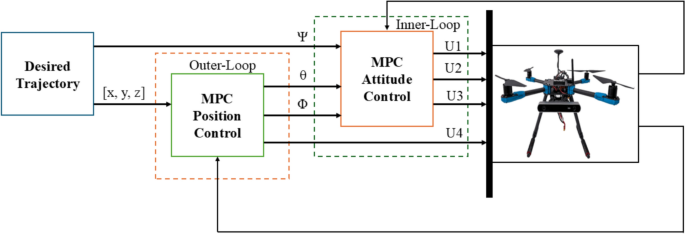
Block diagram of the MPC structure
The proposed cascaded model predictive controller used to fulfil the linear drone dynamics operates through a multi-layered approach. This method involves the implementation of cascade interconnected MPCs, each dedicated to controlling different aspects of the drone’s dynamics to achieve precise and robust performance. Here’s how it works:
- i.In the context of drone altitude control, the altitude controller receives the target altitude () from the trajectory generator, which delineates the drone’s planned flight path. Concurrently, the motion tracking system, utilizing sensors such as GPS or barometers, continuously measures the drone’s actual altitude (). The controller then computes the discrepancy between these two values and determines the necessary thrust input (U1). This thrust input acts as a command signal to the drone’s motors, modulating their power output to achieve and maintain the desired altitude.
- ii.The accelerations in the and directions (horizontal plane) are directly linked to the drone’s rotations. This creates interdependent dynamics, requiring coordinated control mechanisms. Mathematical models (32) and (33) illustrate this relationship, demonstrating that the product of gravity and the respective angle yields a linear displacement. To ensure controlled and safe manoeuvring, the output of the and Model predictive control (MPC) algorithm, which calculates optimal control actions, is constrained within a range of -45° to 45°. These constrained desired angles are then transmitted to the attitude controller for precise execution of the desired flight trajectory.
- iii.The attitude model predictive control system in a drone plays a crucial role in maintaining stable and controlled flight. It receives angular position and angular velocity from the motion tracking system, providing real-time information about the drone’s orientation. Simultaneously, it obtains the desired orientation references from the and MPC algorithm, which have been carefully constrained for safety and stability. By integrating this information, the attitude MPC calculates the optimal torques (U2, U3, U4) required to align the drone’s actual orientation with the desired trajectory. Crucially, this calculation also considers the thrust input (U1), determined earlier in step i, the control process to ensure a holistic approach to flight control.
4.3 PID controller design
A PID controller regulates the control signal using proportional, integral, and derivative actions to maintain consistency between the feedback signal (process variable) and the desired output (set point). The proportional term adjusts the output based on the current error, the integral term corrects steady-state errors, and the derivative term predicts system behaviour by considering the rate of change of error. The following equation describes a common PID formulation:
where:
- Proportional Gain Kp: Scales the instantaneous error between the desired and measured signals to generate the control action.
- Integral Gain Ki : Accumulates the error over time to eliminate steady-state offset.
- Derivative Gain Kd: Responds to the rate of change of the error, adding a predictive component that helps counteract rapid variations.
Together, these gains define the PID controller’s response characteristics for both altitude and attitude control. These specific gains are listed in Sect. 4 (Table 3).
Subsequently, based on Fig. 6 the overall PID control process is described in detail:
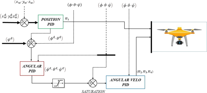
Block diagram of the PID structure (Note. Block Diagram of PID structure is from the article: Sadi, M.A., Jamali, A., Kamaruddin, A.M., & Jun, V.Y. (2024). Cascade Model Predictive Control for Enhancing UAV Quadcopter Stability and Energy Efficiency in Wind Turbulent Mangrove Forest Environment. e-Prime—Advances in Electrical Engineering, Electronics and Energy)
In the quadrotor’s control architecture, the position PID controller receives desired position setpoints () from the trajectory generator and actual position measurements () from the motion tracking system. Based on the deviations between the desired and actual positions, the PID controller calculates the thrust input (U1) for altitude control. Additionally, it determines the desired pitch () and roll () angles to guide the angular PID controller, thereby facilitating precise control of the quadrotor’s horizontal position and orientation. These calculated control signals as shown below (Eqs. 72–74) are then transmitted to the respective actuators to drive the quadrotor’s motion towards the desired trajectory.
where:
: The total thrust force applied by the drone,
: The altitude error, defined as the difference between the desired and actual altitude,
: The proportional gain for altitude control, affecting how strongly the controller responds to altitude error,
: The integral gain for altitude control, compensating for steady-state errors over time, : The derivative gain for altitude control, helping to reduce oscillations by considering the rate of altitude change.
: The vertical velocity, used in the derivative term to smooth altitude control.
where:: : The desired roll angle needed to correct lateral position errors,
: The lateral position error in the world frame,
: The proportional gain for lateral position control,
: The integral gain for lateral position control, addressing steady-state errors,
: The derivative gain for lateral position control, preventing overshoot by considering lateral velocity.
: The lateral velocity of the drone in the world frame.
where: The desired pitch angle required to correct longitudinal position errors,
: The longitudinal position error in the world frame,
: The proportional gain for longitudinal position control,
: The integral gain for longitudinal position control,
: The derivative gain for longitudinal position control,
: The longitudinal velocity of the drone in the world frame.
The angular PID controller subsequently receives desired angular positions , actual angular positions , and actual angular velocities as input signals. Utilizing this comprehensive information, the controller calculates the reference angular velocities required for the PID velocity controllers to achieve the desired orientation as shown in Eqs. (74–76). However, to ensure system stability and prevent abrupt changes in control signals, these reference angular velocities shown below, are constrained within a predefined range, specifically between -45° and 45°. This saturation mechanism ensures smooth and controlled adjustments of the quadrotor’s angular motion, thereby enhancing its overall stability and responsiveness to control commands.
where: : The desired roll angular velocity,
: The roll angle error, difference between the desired and actual roll angle,
: The proportional gain for roll angle correction,
: The derivative gain for roll angle correction, reducing oscillations.
: The current roll rate of the drone.
where: : The desired pitch angular velocity,
: The pitch angle error,
: The proportional gain for pitch angle correction,
: The derivative gain for pitch angle correction,
: The current pitch rate of the drone.
where: : The desired yaw angular velocity,
: The yaw angle error,
: The proportional gain for yaw angle correction,
: The derivative gain for yaw angle correction,
: The current yaw rate of the drone.
The angular PID velocity controller receives as input the desired angular velocities ( calculated in the previous stage, the actual angular velocities () measured by the motion tracking system, and the actual angular accelerations ) also provided by the motion tracking system. Utilizing this comprehensive set of information, the controller computes the optimal angular torques (U2, U3, U4) as shown below in Eqs. (77–79), required to achieve the desired angular motion. Notably, the calculation of these torques considers the thrust input (U1) previously determined by the position PID controller, ensuring a coordinated and integrated control strategy for the quadrotor.
where: : The torque applied to adjust roll angle,
: The proportional gain for roll rate control,
: The derivative gain for roll acceleration correction,
: The roll angle error, : The roll angular acceleration.
where: : The torque applied to adjust pitch angle,
: The proportional gain for pitch rate control,
: The derivative gain for pitch acceleration correction,
: The pitch angle error,
: The pitch angular acceleration.
where: : The torque applied to adjust yaw angle,
: The proportional gain for yaw rate control,
: The yaw rate error.
4.4 Comparison of cascaded MPC and PID control
In this section, a comparison of the cascaded MPC used in our system and PID controller is provided in Table 1. Understanding the differences and advantages of these control strategies is crucial in highlighting the rationale behind our choice of cascaded MPC for controlling the UAV system.