Article Content
1 Introduction
Over 90% of engineering component failures are often caused by fatigue failure [1]. Material fatigue is considered a severe phenomenon where progressive and localised structural damage is applied to a material when it is subjected to cyclic loading or stresses such as tensile, compressive, or torsional [2]. In the materials science and engineering field, it is very crucial to address the issues related to material fatigue as they significantly affect the reliability and safety of various structures and machinery in engineering industries such as aerospace and automotive [3,4,5]. In fracture mechanics, fatigue behaviour is studied with a focus on predicting material failure due to the presence and growth of cracks. Many researchers are investigating the phenomenon of fatigue failures. Many studies have been made to gain more understanding and information about the significance of fatigue failures on material. For example, [6, 7] analysed the fatigue failure issue of a shaft that is used in a wind turbine. The researchers found that the fatigue failure on the shaft was initiated by cracks that are influenced by various variables due to part sizes, loading conditions, and environmental conditions. Besides, based on the study, [8, 9] state that fatigue is considered a mode of failure that causes initiation and propagation of the crack, causing a fracture to occur in the end.
Fatigue failure usually starts initially with a crack in a material, and it affects the mechanical behaviours and structures of a material, causing the performance of the material to transform naturally [10]. The initial fatigue designs rely on the empirical correlations between the nominal stress applied and the corresponding number of cycles, denoted as N, that the structure could endure. Fracture mechanics originated to address and surpass the limitations observed in brittle materials across diverse loading conditions [11]. It is crucial for designers who aim to safeguard structures against catastrophic failure to understand these conditions [12], which mentions that the longevity of material components is quantified in terms of the cycles required for a flaw to propagate and lead to a failure state. Griffith’s work, as mentioned in [13], established that crack propagation demands sufficient energy. A crack may initiate or grow only if the total energy either decreases or remains constant.
With two new crack surfaces being generated, Griffith’s theory posits that materials inherently contain crack-like defects, necessitating energy input to facilitate crack propagation [14]. Consequently, critical fracture conditions denote the point at which crack growth occurs under equilibrium conditions with no net change in total energy. However, this theory needs to be revised to determine the fracture strength of ductile materials. This is due to the substantial plastic deformations experienced by cracked structural metals in the vicinity of the crack tip before eventual fracture. Irwin and Orowan later refined Griffith’s theory by recognising that the accumulated strain energy is expended not only for creating two new crack surfaces but also for the work involved in plastic deformation during ductile material fracture [13]. Based on the studies [15], it was discerned that the energy required to form new crack surfaces in ductile materials is negligible when compared to the work done in plastic deformation at the crack tip. When a crack propagates amidst plastic deformation at the crack tip, there is an expenditure of energy in forming new surfaces in addition to the elastic surface energy [16].
Furthermore, due to the relatively small size of the crack-tip plastic zone compared to the crack dimensions or specimen thickness, the overall elastic strain energy release can still be quantified using elasticity methods [17]. Once the defect size is determined, Griffith’s theory allows for estimating the load that a given structure can withstand. With the load defined, it becomes possible to ascertain an acceptable defect size. As a stress field develops around a crack tip, essential fracture mechanics parameters such as Stress Intensity Factor (SIF) are computed. Crack propagation occurs when the SIF reaches a critical state, with the SIF calculation based on the virtual crack closure technique [18, 19].
Calculating the energy release rate based on continuum two- and three-dimensional FEA outcomes is a commonly used Virtual Crack Closure Method (VCCM). The SIF is determined using the virtual crack extension approach and the energy release rate. The energy release rate is used to compute the VCCM based on the stiffness matrix differentiation at the crack front. Assuming a minimal crack extension, the energy release rate is calculated from the change in potential energy [20, 21]. Since VCCM requires nodal displacement and forces, the energy release rate computation is straightforward when generated in finite element analysis.
It is essential to create modelling for FCG, and various FCG models and software programmes can be used to analyse the FCG model. One of the most used analyses is finite element analysis, which is used for structural analysis and FCG modelling. Finite Element Method (FEM) stands as a robust computational tool for anticipating the behaviour of intricate geometries and structures within engineering applications. The utilisation of the re-meshing technique enhances the capabilities of FEM, enabling the modelling of fatigue crack propagation and the simulation of irregular crack growth through incremental mesh regeneration [22]. FEM is commonly used to predict FCG, but there are difficulties faced during the occurrence of FCG on complicated structures [23]. Based on the studies, [23] stated that the S-version finite element method (S-FEM) can be used to solve the difficulties which are related to the re-meshing process for FCG modelling and complicated crack paths. It is applied for the three-dimensional surface crack issue, and it can evaluate the interactions of multiple surface cracks and the crack closure effect. The presence of surface cracks causes the failure of structural components, and hence, FCG analysis must be carried out. The superimposed FEM, introduced by Fish in 1992, was also employed to enhance FEM’s ability to investigate complex situations with fewer difficulties [24].
Before the S-version method, other techniques, such as the p-method and h-method of finite element platforms, were employed in various investigations, including stress. A common challenge faced by previous researchers lies in the development of numerical methods capable of solving the structure of functions with intricate geometries and high gradients. For instance, regions of high gradients, such as crack propagation, shocks in fluid dynamics, and material failure due to localisation, require numerous elements for accurate resolution. The h-method simplifies the meshing process in the S-version FEM [25], while the p-method increases the polynomial order to enhance accuracy [26]. The h-p version, combining both methods, offers several advantages [25, 27]. This hybrid approach increases the polynomial degree of shape functions and mesh refinement, attracting attention for its potential to secure an exponential number of degrees of freedom [28]. The h-p version aims to build an almost optimal discretisation scheme hierarchically, enhancing accuracy without altering the mesh size [29]. The S-FEM, with its higher-order hierarchical elements superimposed on the original mesh, has been instrumental in improving the quality of finite element calculations in areas exhibiting unacceptable errors.
The FCG model is employed for predicting the fatigue characteristics of certain engineering materials, namely steel, titanium alloy, and aluminium alloy [1]. To analyse and estimate the surface crack growth and propagation that is based on the fracture mechanics, the S-FEM software application is used to carry out numerical analysis in conjunction with multiple FCG models such as the Paris model [30], Frost and Pook model [31], Huang and Moan model [32], and Walker model [33] along with the generation of global mesh and local mesh. A comparison of simulation results based on different FCG models needs to be done to obtain the best model that is the closest to the experiment result. The simulation and experiment results will be addressed after the research is completed. Zhou et al. [34] implemented the FCG models, for instance, Paris’ model, Forman’s model, Elber’s model, Kujawski’s model, Huang’s model, Zhan’s model, and NASGRO model to determine a new FCG rate model by using the machine learning method. Furthermore, Wang et al. [35] and Lee et al. [36] employed FCG models and validated these models using the prediction of fatigue life. Nonetheless, only several models have predicted a good correlation of FCG rate parameters. Most FCG models rely on idealised assumptions about crack propagation, which may not fully capture complex real-world phenomena such as crack closure effects or environmental influences. Alternatively, the FCG models were studied and applied in the analysis using S-FEM software and validated by predicting surface crack growth and fatigue life.
This study focuses on the modelling of FCG. This paper aims to investigate fatigue crack propagation by running the S-FEM simulation together with multiple FCG models. The objectives of the study are to determine the FCG of aluminium alloy materials under bending tests by running the simulation and to analyse the best crack growth model for fatigue cracking assessment. Typically, the FCG forecast is carried out following the identification of the initial fracture [37, 38]. Therefore, this paper focuses on predicting FCG during the stable crack propagation phase, occurring after crack initiation and before unstable crack growth or rapid rupture, based on different types of experiments, number of cracks, materials, and initial crack sizes, as shown in Table 1.
2 Methods and materials
This project involves three aluminium alloy specimens, two of which are Al7075-T6 materials and an AlSi10Mg material. The two types of specimens are selected as they are used for highly stressed structural applications, especially in aircraft structural parts, due to their excellent mechanical properties, flexibility, strength, and fatigue resistance. The dimensions of two Al7075-T6 materials are 140 mm × 65 mm × 25 mm and 150 mm × 60 mm × 20 mm. The dimensions of AlSi10Mg material are 160 mm × 50 mm × 15 mm. The surface crack growth analysis is under two four-point bending models and one three-point bending model that is under crack mode I. The material properties for both aluminium alloy materials are listed in Table 2 and Table 3, respectively. The material properties of both aluminium alloy materials are essential in the S-FEM simulation as they are required to calculate and predict surface crack growth, fatigue life prediction, and SIF. A total of four FCG models are used to predict the surface crack growth in the selected bending models.
For the first four-point bending model undergoing single crack growth, the dimension of this bending model is 140 mm × 65 mm × 25 mm, as mentioned above. Figures 1 and 2 illustrate the geometry of the first four-point bending model and its boundary condition for global mesh and overlaid local mesh.
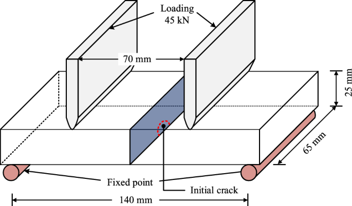
Geometry of four-point bending for Model A
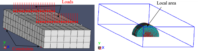
Boundary conditions of global mesh and overlaid local mesh for Model A
Figure 1 shows the model geometry of four-point bending under zero-degree single surface crack in the middle. The material of this model is Al7075-T6, which is commonly used for aircraft structures. The initial crack length and depth are introduced on the notch to produce a semi-elliptical crack shape as the crack growth propagation begins when the bending test starts. The initial crack length and depth are set to 4.5 mm and 3.87 mm. The initial crack size is based on the experimental results.
The boundary conditions for the four-point bending model in the S-FEM simulation are set to be the same as the experiment to ensure that the comparison is valid throughout this project. Figure 2 illustrates the constraints and loadings in the bending mesh model, in which the white dot lines indicate the loadings and the red dot lines indicate the constraints. The fatigue load is applied on the four-point bending model with 45 kN. Figure 2 shows that the local mesh is used to model the pre-cracking area size.
For the three-point bending model undergoing single crack growth, the dimension of this bending model is 160 mm × 50 mm × 15 mm, as mentioned above. Figures 3 and 4 illustrate the geometry of the three-point bending model and its boundary condition for global mesh and overlaid local mesh.
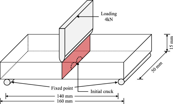
Geometry of three-point bending under multiple surface cracks for Model B
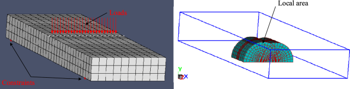
Boundary conditions of global mesh and overlaid local mesh for three-point bending for Model B
Figure 3 shows the model geometry of three-point bending under zero-degree single surface crack in the middle. The material of this model is AlSi10Mg, which is commonly used for aircraft structures as well. An initial crack length and depth are introduced on the notch to initiate the crack growth propagation when the bending test starts to produce two semi-elliptical crack shapes. The middle of the bending model is designed to be the origin, and the position of the left notch is placed 4 mm to the left, and the right notch is placed 5.5 mm to the right. The initial crack lengths and crack depths for the left surface crack and suitable surface crack are set to be 5.5 mm and 3.84 mm, and 3.5 mm and 2.42 mm. The initial crack size is based on the experimental results.
For this three-point bending model under two surface cracks, the boundary conditions in S-FEM simulation are set to be exact as the experiment to ensure the comparison between experimental data and simulation data is accurate and valid throughout this project. Figure 4 displays the constraints and loadings in the bending mesh model, in which the white dot lines indicate the loadings and the red dot lines indicate the constraints. The material used in this bending model is AlSi10Mg, and the fatigue load is set as 4 kN, and it is applied on the three-point bending model. Figure 4 shows the local mesh that modelled the size of the pre-cracking area. After the required setup is done in the S-FEM simulation, the results are extracted from the simulation, and the analysis is conducted and explained in detail below.
2.1 Simulation method
This section will discuss two topics: the formulation of the S-FEM concept and FCG models. Formulations and matrices of equations related to FCG analysis will be covered that are based on the stress analysis concept. The stiffness matrix is determined after considering stress–strain and strain–displacement relations. The discussion will centre on the formation of a three-dimensional stress analysis issue. This section also focuses on the concept execution of S-FEM in crack surface analysis. The mathematical formulations related to the S-FEM will be discussed in detail, together with various FCG models. The equation of stress–strain equation is formulated as follows:
where σ represents the stress matrix, [D] represents a matrix of material properties, and represents the strain matrix. Following the equation of strain–displacement that is given by:
The deformation matrix and the displacement matrix are both represented by [B] and . Meanwhile, Eq. (3) is formulated by substituting Eq. (2) into Eq. (1), and it is shown as:
The relation between stiffness [k] and loading [F] matrices produces displacement {u}, and the force [F] is expressed as follows:
The stiffness [k] is formulated as follows:
The for global element and for the local element. The element stiffness and force can be identified as shown below since the equation
As a result, Eq. (7) can be written as follows:
Then, finite element formulation can be expressed in matrix form, which is:
The matrices at Eq. (8), and are the stiffness matrices of the merging area. and represent the nodal forces in global and local regions. The relationship between and is shown below:
The strain displacement matrix in the global region is replaced by , where the integration of Gauss points is considered during the overlay process between local and global regions. A Gauss point is an integration point within an element where integrals are numerically evaluated. Each element, both local and global, has its coordinate system. For implementation in this S-FEM, the three-dimensional element is computed. The notations (L) and (G) represent local and global, respectively, where the coordinates are derived from the transformation of the local coordinates .
As the general finite element and S-FEM concept formulation are discussed in the last section, this section focuses on the investigation of the origin of the energy release rate and SIF following the derivation of formulas for the nodal displacement of the elements and stiffness matrices on the overlaying region. FCG applies the application of energy release rate and SIF from the behaviour of crack propagation described by the linear elastic fracture mechanics (LEFM).
In this investigation, a commonly used method, which is the virtual crack closure method (VCCM) in three-dimensional finite element analysis, is used to evaluate the energy release rate, G and SIF, K [45]. It is assumed that the arrangement of the crack plane finite element mesh is in an orthogonal manner, and the mesh sizes across the crack front are required to be equivalent. [45] describes the energy release rate formula at the crack front segment is given by:
where the element’s width and length correspond to parallel and perpendicular to the crack front, and J indicates the segment number along the crack front. The values σ are the cohesive stresses in the plane of the crack ahead of the crack front, while are the crack opening displacements as a function of the distance from the crack front. denotes the area of the face of a finite element at segment J of the crack front. It is important to note that the coordinates and are perpendicular and parallel to the crack front, respectively, and the axis is normal to the plane of the crack. refers to the total energy release rate.
The calculation of the energy release rate leads to the calculation of the SIF based on different crack mode loadings as follows:
Hence, in the context of planar stress, Young’s modulus of elasticity is E. The energy release rate, , i = {I, II, III} will be obtained based on different crack front scenarios and used in crack growth simulation since the failures occur in the region of linear elastic fracture mechanics.
With the adoption of 20 node hexahedron element, the nodal forces, and the nodal displacement differences between upper and lower crack faces, , are used for the VCCM calculation where indicate the nodal points on the crack plane. The formula of VCCM is updated as follows:
The constant can be expressed as follows:
Depending on the mixed mode problems according to the three crack mode loadings, which are mode I, mode II, and mode III, the total energy release rate, , can be separated into its sections, which are , , and as:
The detail of a specific condition at the crack front arrangement for the implementation of VCCM could be referred to Okada et al. [20]. When the crack is opened for one element, the mode I component is considered, and the energy release rate, , spent on the crack area, , can be evaluated as follows:
Symbol and represent the length and width, which are perpendicular and parallel to the crack front, respectively. σ indicates the cohesive stress in the crack’s plane that is located before the crack front. The cohesive stress is designated by 33, with the vertical face being represented by the first number and the horizontal face being represented by the second number of axes. The function represents the crack opening displacement. The symbol stands for Young’s modulus, and represents Poisson’s ratio. The variable shows the distance from the crack front , and the angle between the , the angle between the direction and the crack front’s average direction is represented by . In this context, equals for plane stress, and equals for plane strain. The cohesive stress, σ, and the displacement function at the crack that are substituted into the extended formula of can be interpreted as follows:
The crack segment areas, and , can be expressed by:
From Eq. (12), the SIFs, based on different crack mode loadings, are expressed by its energy release rate, , implemented by [45], can be expressed in terms of for and as follows:
From the calculations of energy release rates, the equivalent SIF, , can be obtained through Eq. (12). The crack growth rates from various FCG models can be calculated with , which will be covered and discussed in the next section. Furthermore, the crack growth angle can be calculated with the influence of the , , and values via Eq. (12) [46] as follows:
where the crack growth angles are and .
The four FCG models used in this study are as follows: The formulas of each model are discussed below to show the differences between them for S-FEM simulation. The Paris model [30] describes a popular method based on a power law known as Paris Law for predicting crack growth propagation. The Paris law is user-friendly and involves determining two easily obtainable curve-fitting parameters. This law is frequently applied if the data exhibit a linear relationship.
The fatigue rate curve’s region II is described by the equation above, which shows a straight line on the log–log plot of (da/dN) versus (ΔK), where c is the Paris model constant, which is the intercept, and n is an exponent which is the slope on the log–log plot of (da/dN) versus (ΔK). The FCG data is analysed to predict fatigue life by generalising the Paris relation [47].
For Frost and Pook’s model, in their efforts to formulate an FCG equation with meaningful physical implications, [31] proposed a hypothesis. They suggested that under cyclic loading, crack growth does not result from progressive structural damage but instead occurs because unloading reshapes the crack tip at each cycle. According to this sequence, the formation of striations is attributed. Consequently, the increase in crack growth during each cycle can be linked to the alterations in crack-tip geometry as it undergoes opening and closing. Their proposal is based on a straightforward model.
Plotting the prediction from the planar stress equation versus (da/dN) in terms of (ΔK/E) shows that it agrees well with the experimental data, especially for crack growth rates of about (3 × 10⁻⁵) mm/cycle. Nevertheless, experimental crack growth rates are overstated at low and underestimated at high growth rates.
The Huang and Moan model [32] proposed a unified R-ratio formula that introduces an additional parameter, denoted as M, within the − 5.0 < R < 1.0 range. M serves as a correction factor distributed across three distinct R-ratio ranges, aiming to align FCG curves of various R-ratios with the curve corresponding to R = 0. The parameter β varies based on the material and is determined by fitting the results of fatigue tests.
where β and β1 are parameters depending on the material property and environment (β ≤ β1 < 1); constant C and exponent n are depending on the material properties. The current model suggests that the exponent n, representing the crack growth rate, is presumed to be unaffected by the R-ratio. When calculating fatigue life under various R-ratios, the necessary material constants C and exponent n can be directly derived from the constants associated with any specific constant R-ratio [48].
For the Walker model, the primary constraint of the Paris model is its incapacity to consider the stress ratio. Recognising this limitation, [33] sought to enhance the Paris model by incorporating the influence of the stress ratio. Walker introduced a parameter, representing an equivalent zero-to-maximum (R = 0) SIF that induces the same growth rate as the actual combination of and R.
The importance of this equation lies in the fact that a log–log plot of da/dN versus ΔK should yield a singular straight line, irrespective of the stress ratio from which the data were derived. The inclusion of a third curve-fitting parameter, , allows for the adjustment needed to consolidate the data into a single straight line on the log–log plot of da/dN versus ΔK. The determination of involves trial and error, with the selected value being the one that optimally aligns the data along the desired straight line. It is important to note that there might be cases where no suitable value of can be found, rendering the Walker equation inapplicable. When equals one, is equivalent to , signifying that the stress ratio has no impact on the data. In summary, as an adaptation of the Paris law, the Walker law accommodates the stress ratio effect at the cost of introducing a third curve-fitting parameter [48].
2.2 Experimental method
An Instron dynamic system was used to perform the four-point and three-point bending fatigue tests. Both dynamic and static testing environments may be used with the 8874 servo-hydraulic fatigue testing equipment, which can execute a fatigue test with a load of up to ± 100 kN. This completely digital servo-hydraulic controller may automatically calibrate all the suitable transducers. The controller is accessed through the console software. A transducer’s calibration necessitates a few interface procedures. The controller automatically detects the characteristics of the load cell or extensometer when it is changed and stops the test from commencing until the calibration has been calculated. A strain gauge load cell is used to calibrate the force amplitude.
According to the previous research, the frequency had been set at 20 Hertz for all experimental conditions [29]. The three-point and four-point bending model specimens were positioned in the middle of the rigs, as shown in Fig. 5. The specimen’s geometry could have been used to modify the upper and lower rigs. With the surface fracture facing the lower test rig, the specimen was placed in the centre of the rig. The upper test rig was changed to switch to the four-point bending model. The lower rig was gradually adjusted until the force transducer displayed a value of zero or almost zero after the specimen had been positioned by the necessary guidelines. This was done to guarantee that the specimen was secured and that loading could be applied straight to the body.
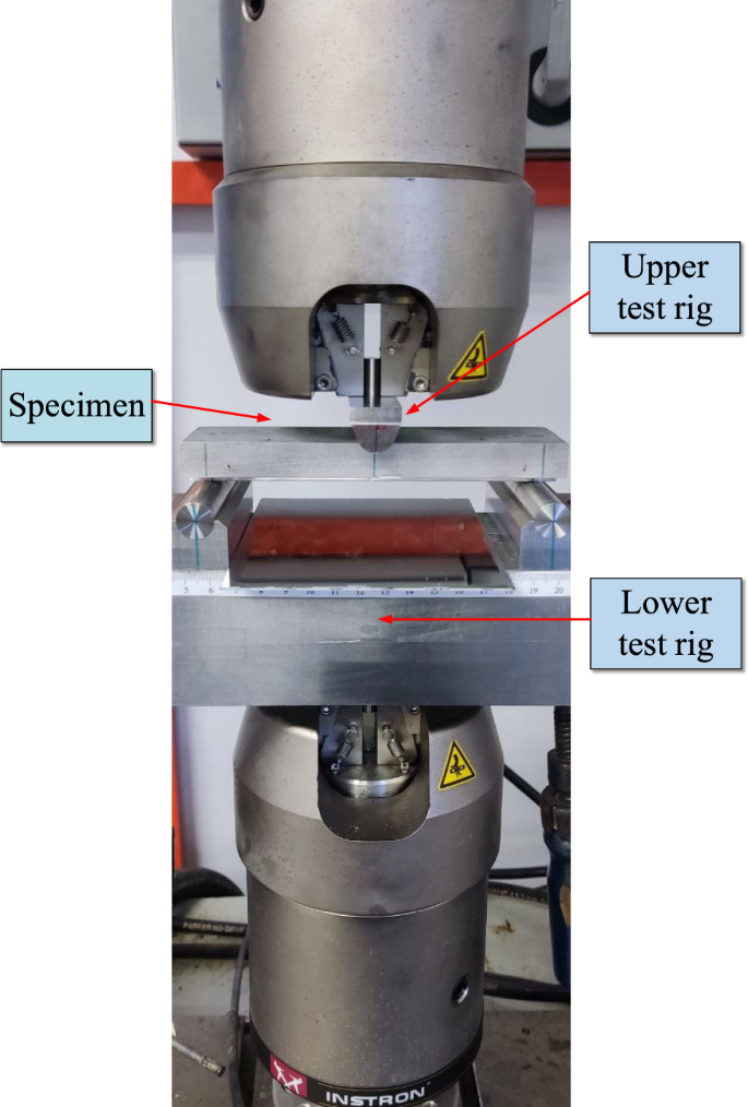
Specimen positioned in the middle of the upper and lower test rigs
The user was able to specify the loading history using the WaveMatrix™ automated settings, which allowed the entire experiment to run continually. In order to satisfy the expectations of researchers, the Instron servo-hydraulic testing equipment is outfitted with a variety of sensors and accessories. A force and displacement transducer is one of them. Users may implement and monitor the loading with the help of the force transducer. Nevertheless, the displacement will replace the force as the input if the user prefers to utilise it for the experiment. Users can additionally customise the motion type using the WaveMatrix™, including random, square, and sinusoidal motion. The constant amplitude loading was replicated in this study using a continuous sinusoidal wave.
The loading history of the investigation was subsequently set up using the WaveMatrix™ programme, as shown in Fig. 6. The tester considered the process simple to use the programme to generate the loading because to the user-friendly graphic interface. The loading history was subsequently developed with a stress ratio (R) of 0.1 for the crack propagation and 0.8 for the benchmarks, with maximum stress (Fmax) set at 4 kN for the three-point bending model and 45 kN for the four-point bending model. The minimum load would be 0.4 kN and 4.5 kN, with a maximum load of 4 kN and 45 kN and a stress ratio of 0.1. The mean stress was identified to be 2.2 kN and 24.75 kN. The loading history that was supposed to generate the benchmarks is shown in Fig. 6. This procedure was repeated for up to 20,000 cycles and 100,000 cycles, respectively, and stress ratios of 0.1 and 0.8 were tested. When the specimen was fractured entirely, the fatigue test was discontinued. Figure 7 depicts the entire experimental procedure.
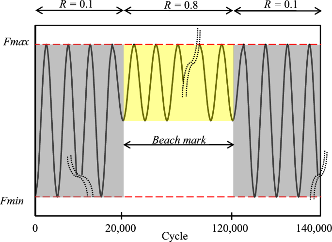
Amplitude of cyclic loading
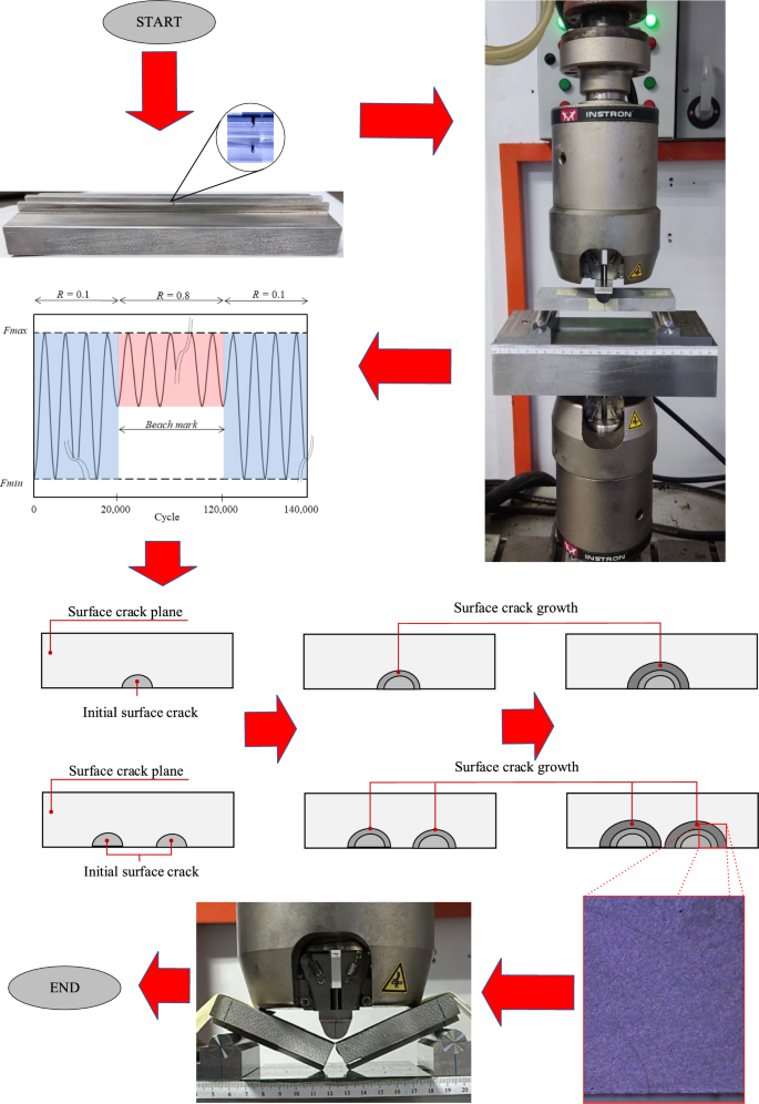
Experimental process
Finally, the coordinates were plotted, and the number of cycles was calculated. Plotting the experimental and S-FEM data on the same graph allowed for the results to be confirmed. Additionally, the failure cycle was verified to demonstrate the S-FEM’s capabilities.
3 Results and discussion
The results and discussion of the S-FEM simulation with four selected FCG models are presented in this section. It is essential to verify the accuracy of simulation results by comparing experimental data to identify the best FCG model. The experiment data can decide the precision of an FCG model within its acceptable range by using the root-mean-square error method to validate the results. Table 1 shows the information of all models according to different types of experiments, cracks, material, and experimental results. The models consisted of two models: Model A and Model B. The following subsections compare simulation results with experimental data in detail based on three sections: surface crack growth, fatigue life prediction, and SIF.
3.1 Surface crack growth
This section covers the surface crack growth analysis under two four-point bending models and one three-point bending model under crack mode I. Four FCG models are used to predict the surface crack growth in the selected bending models.
For the single surface crack growth with a four-point bending model, it is found that the simulation results of crack growth propagation for the Paris model, Walker model, and Huang and Moan model are similar to each other except for the Frost and Pook model. There are 30 beachmarks set for the simulation to run for the crack growth propagation, and the mean beachmarks from the simulation are around 22–23. Meanwhile, only five beachmarks were obtained from the experimental data. The distances between each beachmark represent the crack length, c, and crack depth, a, and the beachmarks from the four-point bending test and multiple FCG models are compared in graphs to display the differences in crack length and crack depth.
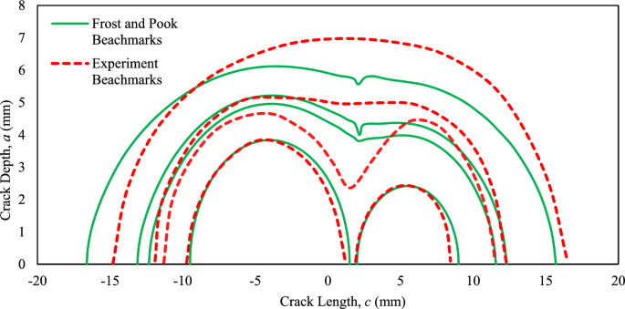
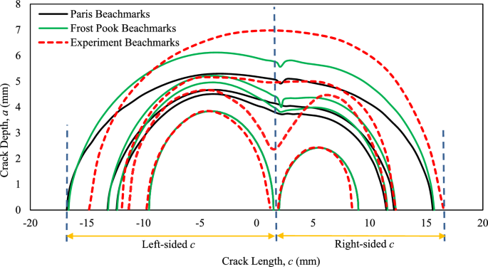
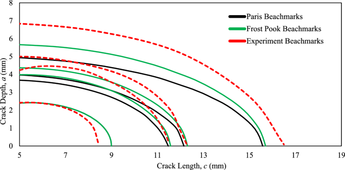
Figure 8 illustrates the comparison of crack growth propagation between experimental data and simulation data of the Paris model. Figure 9 displays the comparison of crack growth propagation between experimental data and simulation data of the Frost and Pook model. Figure 10 shows the comparison of crack growth propagation between experimental data and simulation data of the Paris model and the Frost and Pook model. Figure 11 displays the graph of the four-point bending experiment vs the Paris model and the Frost and Pook model that is focused on right-sided c. The differences between every beachmark between the Paris model and the Frost and Pook model are almost similar compared to the beachmarks from the experimental data. The differences show that the crack growth propagation prediction of simulation is similar and near to the actual crack growth propagation of aluminium alloy 7075-T6 from a four-point bending experiment.
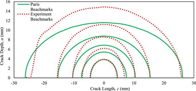
Surface crack beach marks of four-point bending experiment versus Paris model for Model A
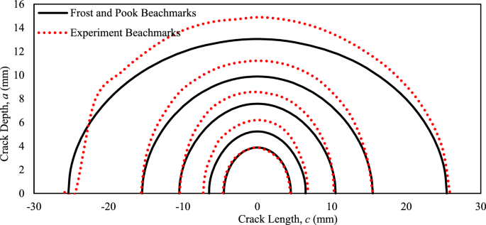
Surface crack beach marks of four-point bending experiment vs Frost and Pook model for Model A
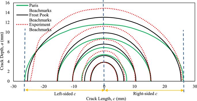
Comparison of surface crack growth beach marks predictions for Model A
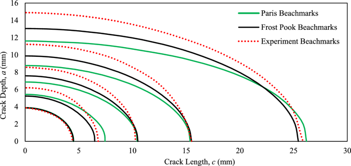
Comparison of surface crack beach marks for Model A. Focus on the right-sided c
To validate the differences of crack length, c, between experimental data and predicted data from two FCG models, an error measurement method, which is root-mean-square error (RSME), is introduced to calculate the difference between values predicted by a model and the actual values. The formula of RMSE is given by:
where the and indicate the actual data value and predicted data value, represents the total number of data, and variable is dependent on the N. Table 4 shows the calculation RMSE and the final values of the RMSE regarding the two FCG models. The difference between right-sided c between the experiment and two FCG models is used for RMSE calculation. Table 4 shows that the RMSE values for the Paris and the Frost and Pook models are 0.3318, 33%, and 0.2624, 26%, respectively. The lower the RMSE values, the higher the accuracy of the FCG model data to the experiment data. Frost and Pook’s model has lower RMSE values, which indicates that the model is better at predicting surface crack growth propagation than the Paris model.
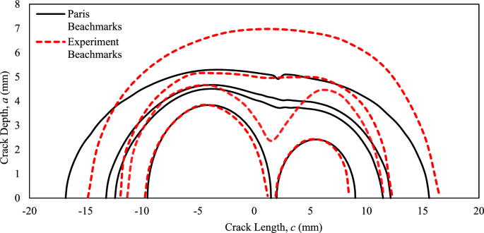
For the two surface crack growth under the three-point bending model, it is found that the simulation results of crack growth propagation for the Paris model, Walker model, and Huang and Moan model are similar to each other except Frost and Pook model. There are 15 beachmarks set for the simulation to run for the crack growth propagation, and the mean beachmarks from the simulation are around 15 times the total beachmarks that the S-FEM simulation completed the pre-set. However, the Frost and Pook model on three-point bending multiple surface cracks simulation was only able to obtain 13 beachmarks. This may significantly affect the comparison result, which is discussed in detail below. Meanwhile, only five beachmarks were obtained from the experimental data. The distances between each beachmark represent the crack length, c, and crack depth, a, and the beachmarks from the three-point bending test and multiple FCG models are compared in graphs to display the differences in crack length and crack depth.
Figure 12 illustrates the multiple crack growth propagations from the simulation data of the Paris model. A total of five beachmarks were obtained from the three-point bending experiment. Figure 13 displays the multiple crack growth propagations from the simulation data of the Frost and Pook model. A total of five beachmarks were obtained from the three-point bending experiment. Figure 14 compares crack growth propagation between experimental data and simulation data of the Paris and Frost and Pook models. Figure 15 shows the graph of the three-point bending experiment versus the Paris model and the Frost and Pook model, which is zoomed in on the right side of crack growth propagation. The differences between every beachmark of the Paris and the Frost and Pook models are almost similar compared to the beachmarks from experimental data. The differences show that the simulation’s crack growth propagation prediction is similar and near to the crack growth propagation of aluminium alloy AlSi10Mg from a three-point bending experiment.
Multiple surface crack beach marks of Paris model on three-point bending versus experimental data for Model B
Multiple surface crack beach marks of Frost and Pook model on three-point bending versus experimental data for Model B
Comparison of the multiple surface crack beach marks for Model B
Comparison of surface crack beach marks for Model B. Focus on the right-sided c
The root-mean-square error (RSME) was calculated for the differences in crack length, c, between the experimental data and predicted data from two FCG models for Fig. 15. The root-mean-square error (RSME) was calculated based on Eq. (35). Table 5 displays the calculation of RMSE and the final values of the RMSE regarding the two FCG models.
Table 5 shows that the RMSE values for the Paris and the Frost and Pook models are 0.5457, 55%, and 0.4887, 49%, respectively. The lower the RMSE values, the higher the accuracy of the FCG model data to the experiment data; the Frost and Pook model is more suitable to predict the multiple surface crack growths based on its lower RMSE values, which indicates that the model is better to predict the surface crack growth propagation compared to Paris model. The analysis of fatigue life prediction will be discussed in a further subtopic.
3.2 Prediction of fatigue life
This section focuses on analysing fatigue life predictions from multiple FCG models with a comparison to the experiment data. It is significant to predict the fatigue life of a material when it handles different loadings by determining the number of failure cycles until a fracture occurs. The life of crack formation and propagation on a material can be equivalent to its fatigue life [49]. The bending models involve a three-point bending model and a four-point bending model, and there are two materials used for the bending models, which are aluminium alloys Al7075-T6 and AlSi10Mg.
This section contains two four-point bending models with the material Al7075-T6 and one three-point bending model with the material AlSi10Mg. Several graphs are presented to compare the FCG models on S-FEM simulation with the experiment results.
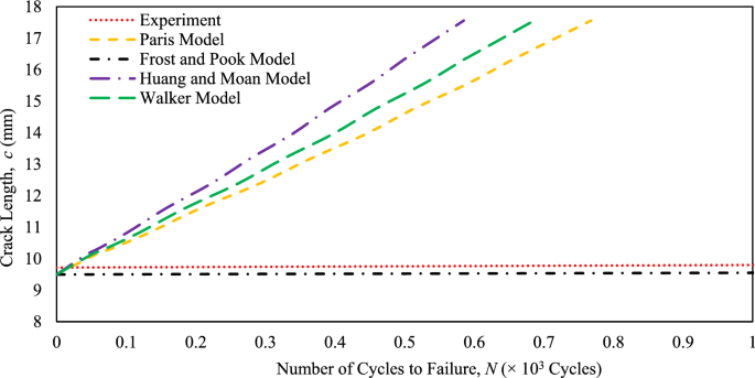
For the first four-point bending model with Al7075-T6 material, Fig. 16 shows the graph of crack depth, a vs number of cycles to failure, N with all the selected FCG models and experiment data. The crack depth data for each FCG model and experiment are obtained by measuring the distances of each beachmark on the y-axis. After the crack depths are measured for the experiment and all the models, the number of cycles to failure is obtained for plotting the graph in Fig. 16. The number of cycles to failure for FCG models is calculated in the simulation S-FEM application, whereas the number of cycles to failure for the experiment is collected throughout the four-point bending test. As shown in Fig. 16, it is noticeable that the Frost and Pook model is the nearest to the experiment in the low cycle area, which is lower than 300 Kilocycles; this indicates that the Frost and Pook model is the best FCG model in low cycle area for crack growth prediction in this bending model. Meanwhile, as the number of cycles to failure exceeds 300 Kilocycles, the Paris model is the best FCG model for this bending model to predict the FCG as it is the closest to the experiment.
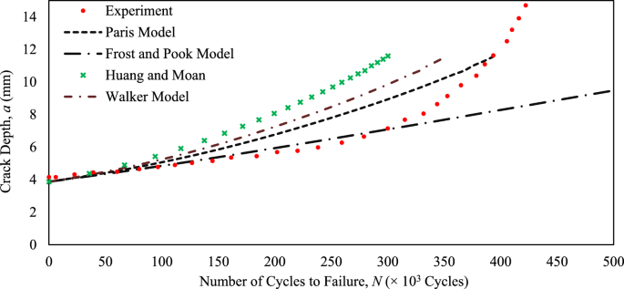
Fatigue life cycle to failure for Model A
Next, from the three-point bending model, as illustrated in Fig. 3, multiple graphs of crack length with a number of cycles to failure are plotted to analyse the prediction of fatigue life from FCG models. Figures 17 and 18 are presented to show the comparison of left-sided and right-sided crack length with failure cycles, number of experiments, and multiple FCG models.
Graph of left-sided crack length, c vs failure cycle numbers, N with N capped at one thousand cycles for Model B
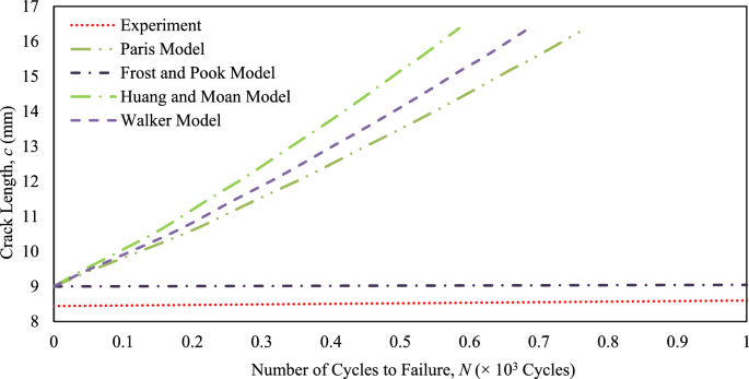
Graph of right-sided crack length, c vs failure cycle numbers, N with N capped at one thousand cycles for Model B
The crack lengths from the left-sided and right-sided on this bending model are used to plot the fatigue life graphs with a number of cycles to failure from four FCG models. The experimental data for this three-point bending model are used to compare with multiple FCG models. From Figs. 17 and 18, it is observed that the number of cycles to failure for the Paris model, Walker model, and Huang and Moan model ranges between 0.55 Kilocycles to 0.85 Kilocycles, which is considered further from the failure cycle numbers for the experiment that is around the maximum value of 60 Kilocycles. The experiment and Frost and Pook model show a flat line since the crack propagation is minimal. Meanwhile, the Frost and Pook model has the highest number of failure cycles, which is beyond 80 kilocycles, with crack lengths similar to those of other FCG models. The specimen was fractured at 60 Kilocycles during the experiment. The predicted fatigue life of the Frost and Pook model is the closest compared to that of the experiment, and it indicates that the prediction of crack propagation is considered accurate for real-life applications.
3.3 Stress intensity factor
The intensity of stress at the crack front or tip can be assessed through the SIF. SIF evaluates the possible crack propagation and enlargement from an existing crack. This section only covers the four-point bending model with the material Al7075-T6. The SIF values are obtained from the simulation of S-FEM with multiple FCG models such as the Paris model, Frost and Pook model, Walker model, and Huang and Moan model. However, the SIF value from the bending test experiments cannot be obtained directly to compare with that from the simulation as SIF requires its formula to calculate, which is easily accomplished by using numerical methods available in the S-FEM simulation. The values of critical SIF and of materials, Al7075-T6, are introduced to validate the SIF values from the simulation and investigate the possible catastrophic failure. Several graphs are plotted for bending models to illustrate the values of SIF over crack angle, and they are discussed in detail based on the graph pattern.
Figures 19 and 20 display the SIFs of the single surface crack four-point bending model from the Paris and Frost and Pook models. As the surface crack growth of the Paris model is the same as that from the Walker model and Huang and Moan model, the Paris model is represented to present the SIF graph to compare with the Frost and Pook model. It is observed that the graph of SIF over the crack angle is normal and acceptable, as both SIFs do not exceed the , which is 30 Mpa.√m, so there is no catastrophic failure when the load is applied.
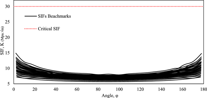
SIFs of single surface crack four-point bending Model A from Paris model
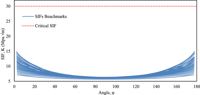
SIFs of single surface crack four-point bending Model A from Frost & Pook model
4 Conclusion
S-FEM concepts are applied in the simulation to calculate and predict the surface crack growth and propagation. Multiple FCG models are used in S-FEM simulation to obtain simulation results that can be compared with the experimental results. The objectives of this study are achieved as the FCGs of aluminium alloy materials under bending tests involving the three-point bending model and four-point bending model are successfully determined with the simulation, and they are validated with the experimental results to prove the FCG models are helpful in the engineering analysis. Furthermore, after various studies, including surface crack growth, fatigue prediction, and SIF calculation, the best FCG model was identified based on the surface crack quantity and bending models. Frost and Pook’s model is considered the best for predicting and estimating the FCG propagation based on the analysis from this research on three- and four-point bending tests. The fatigue life prediction using the Frost and Pook model is more closely related to the experimental results than other models. Furthermore, the prediction of surface crack growth is noticeable with the lowest RMSE value in four three-point bending and four-point bending models with 26% and 49% error by using the Frost and Pook model.