Article Content
1 Introduction
The bogie frame is a structure that supports the loads of the vehicle body, limits the motion of the wheelsets, and is a fundamental part of the suspension design. This critical component motivates frequent visual inspections to allow the early detection of damage. Crack initiation and other types of damage may be caused by defective manufacturing or factors related to the railway operation [1]. The vehicle–track interaction is characterized by high dynamic forces [2], including impacts, that promote the mutual damage of the bogie components [3] and the infrastructure [4]. Therefore, there is a potential benefit on complementing visual inspections with online condition monitoring techniques, that can also be used to monitor the overall railway dynamics, including the vehicle stability [5] and wheel damage [6, 7].
Most of the literature concerning the bogie frame condition focuses on the prediction of its remaining life [8,9,10,11]. On the contrary, the available literature concerning the real-time monitoring of the condition of the bogie frame is rather scarce. The existing techniques used to detect the development of fatigue cracks are mostly limited to the use of elastic-guided waves (EGW), that involve the use of forced, prescribed vibrations [12]. Yan et al. [13] show that EGW can be used to detect a small crack in a specimen using a sensor network in the vicinity of damage. Hong et al. [14] propose the use of a system of actuators/sensors that simultaneously generate and measure the EGW transmitted by the bogie frame. The local differences between the reference emitted signals and the measured signals, caused by changes in the amplitude, delay, and scattering of the EGW, allow the damage detection and identification. However, this approach requires a large number of sensors distributed on the bogie frame to deliver a signal powerful enough to travel through the thick elements of the structure. Zhang et al. proposed a similar approach using EGW to detect and isolate bogie frame cracks [15].
The understanding that damage modifies the vibrational behavior motivated the development of several condition indicators, using the FRFs and the transmissibilities measured between different points of a structure [16,17,18,19]. The response assurance criterion (RVAC) [20] is originally defined as the correlation, at a given frequency, between the undamaged and damaged operational deflection shapes (ODS) of a structure. The detection and relative damage quantification indicator (DRQ) [21] collects the contributions of the different values of the RVAC in the frequency range of interest and normalizes those contributions by the number of frequencies considered. The transmissibilities can be used instead of the ODS to define an alternative form of the RVAC for a given frequency. In the context of single degree of freedom (SDOF) systems, the transmissibility is commonly defined as the ratio between the amplitude of the response and the amplitude of the imposed motion, assuming harmonic motion. Similarly, it is defined in terms of forces, as the ratio between the transmitted and applied force in SDOF systems [22]. The concept of transmissibility is first presented by Ribeiro et al. [23] and further extends to systems with multiple degrees of freedom. The transmissibility matrix is originally defined using the Frequency Response Functions (FRFs) of the structure, expressed in the form of the receptance matrix, or directly, using the measured responses. This work applies the concept of direct transmissibility [24], defined as the ratio between the response of any two points of a structure. Fontul et al. [25] show that the original relationships formulated assuming harmonic or periodic motion can also be applied to random inputs. In the case of random excitation, the transmissibilities are evaluated relating the spectral densities of the responses at different points of the structure. Accordingly, the Transmissibility Damage Indicator [26], in analogy to the DRQ, compiles the contributions from the RVACs defined using the transmissibilities and normalizes them by the number of frequencies. The Maximum Occurrences method [27, 28], also called Frequency of Maximum Differences method, is an algorithm that can support the localization of damage by highlighting the pairs of points on the structure where TDI is the most sensitive to changes in the response of the structure.
In a previously published work, Millan et al. successfully applied a methodology using the concept of transmissibilities to detect the failure of springs of a railway locomotive [29]. The authors proposed the Localized Transmissibility Damaged Indicator (LTDI), which showed promising potential to detect spring failure. The LTDI is a particular case of the TDI, limited to the transmissibilities between pairs of measuring points which, in the context of the locomotive suspension elements, may be the ends of the springs that are monitored. Using a detailed model of the locomotive, the vehicle response is obtained through the simulation of the vehicle–track interaction, using the general-purpose multibody software MUBODyn [30,31,32,33].
Solutions presented in the literature for the condition monitoring of bogie frames bear relevant limitations that this work aims to address. The indirect assessment of the structural condition using load profile evaluations to estimate the accumulated stresses [8,9,10,11] is subjected to the limited accuracy in the measurement of the forces applied on the bogie frame, and the inability to detect the sudden failure of the structure in a timely manner. The direct assessment of the condition using EGW [12,13,14,15] involves the distribution of force actuators in a large enough number that is capable to excite the structure, while countering the attenuation effects that hinder the detection and localization of damage by the large sensor system that must also be installed. Alternatively, the present work proposes the development of an online damage detection and localization strategy for the bogie frame of a locomotive that can be applied during the regular railway operation. This approach involves the measurement of the structural vibrations that result from the vehicle–track interaction during the operation, and the application of the concept of direct transmissibilities to identify changes in the bogie frame response that can be attributed to the structural damage. This strategy dispenses the estimation of the load profile, or the need to excite the structure artificially with forced vibrations. The investigation of the feasibility of the TDI and MO to detect and localize bogie frame cracks, directly using the structural vibrations, and the analysis of the effects of uncertain operational parameters on the condition indicators are novel contributions of this work that the authors hope to contribute to enhance the state-of-art of condition monitoring in the railway context.
2 Methods
2.1 Direct transmissibility
The direct transmissibility, also called local transmissibility, is defined as the ratio between the amplitudes of the responses at any two points of a structure, expressed by:
where τrs is a scalar quantity, Xr and Xs are two known scalar amplitudes, and r and s are indices that identify measurement coordinates on the structure. Maia et al. demonstrate that, in general, the direct transmissibilities depend on the magnitudes and points of application of the forces on the structure [24]. Consequently, the direct transmissibilities of a system subjected to two significantly different load scenarios are not comparable. Nonetheless, in the railway context, the points of application of the loads in a bogie frame do not change, and this work proposes conditions that validate the assumption that the load spectrum is constant.
2.2 Damage detection using transmissibilities
Damage changes the modal properties of a structure, disturbing its vibrational behavior. In turn, the changes in the vibrations affect the transmissibilities between certain locations in the structure. Damage detection techniques using transmissibilities associate the changes in the transmissibilities, relative to a reference case, to assess the condition of the structure.
2.2.1 Transmissibility damage indicator
The Transmissibility Damage Indicator (TDI), proposed by Maia et al. [26], is an approach developed to detect and quantify structural damage. The development of TDI is inspired by the Response Vector Assurance Criterion (RVAC), defined by Heylen et al. [20] as the correlation between the frequency response functions of the undamaged and damaged structures, for a given frequency. Contrary to other condition indicators, the TDI avoids a previous modal identification of the structure. Additionally, the TDI does not require the precise knowledge of the forces involved and, under the assumption that the points of application of the forces and the force spectrum are constant, depends only on the structural response. The transmissibilities can be evaluated in the frequency domain using the power spectral density (PSD) of the responses.
Matrix τn(ω) is defined by the direct transmissibilities between all the N measured points of the structure in nominal condition, as a function of the frequency ω, according to:
Likewise, matrix τd(ω) expresses the direct transmissibilities of the structure in the unknown condition. For simplicity, hereafter τn(ω) is called the nominal condition matrix, while τd(ω) is the damaged condition matrix. These are not to be mistaken by the transmissibility matrices, as they are defined throughout the literature. The Response Vector Assurance Criterion (RVAC) can be adapted to express, for each frequency, the correlation between the values of the local transmissibilities of the undamaged and damaged structures [26]. Considering M points of application of forces on a structure and a sequential progression of the evaluation of the transmissibilities over the N points of the structure, given by s = r + 1, the RVAC is expressed by:
However, if the location of the points of application of the forces on the structure do not change, the RVAC can be simplified to:
The TDI is a normalization of the contributions of the RVAC over Nω frequencies of interest, following:
The TDI values vary between 0 and 1. Values close to unity show there is a strong correlation between the nominal condition and the measured response, meaning that the structure is healthy. Lower TDI values suggest the structure is damaged. The sequential scheme between the measurement points of the structure, presented in the original formulation, is simply defined by:
meaning the transmissibilities are evaluated in successive pairs of points in increasing order of the indices that identify them. However, this progression is not adequate if the geometry of the structure is complex or intricate, because there is no evident way to define such a sequence that is general enough to be applied to a large variety of load scenarios and damage locations. This fact motivated the development of an alternative expression concerning how the transmissibilities of the different measurement points of the structure are correlated. Considering the transmissibilities of all the measurement points in the structure are involved in the calculation of TDI, the symmetric scheme is defined by the expression:
In terms of the condition matrices, this means relating all the entries of the matrices, except the entries in the main diagonal. The expressions in Eqs. (5) and (7) will be used henceforth in this manuscript.
The use of the TDI method to assess the condition of structures relies on the processing of the response according to the methodology depicted in Fig. 1. The signals in the time domain, in general accelerations, velocities, or displacements, are transformed to the frequency domain using PSD estimates of those signals. The PSDs of the structure in nominal condition, that represent the nominal response, are combined to define the nominal condition matrix τn(ω), which is a three-dimensional matrix that is a function of the frequency ω and the indices r and s of the measurement points. Conversely, the PSDs of the structure in the unknown condition are used to define the damaged condition matrix τd(ω). Finally, τn(ω) and τd(ω) are compared to compute the TDI.
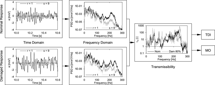
Condition monitoring methodology using the TDI and MO methods (adapted from [29])
2.2.2 Maximum occurrences
The Maximum Occurrences method, also called Frequency of Maximum Differences algorithm, is proposed by Sampaio et al. [27, 28] for the localization of damage, after proper damage detection is achieved. For each frequency, the condition matrices τn(ω) and τd(ω) are used to compute the subtraction:
and the entry with the highest absolute value of the matrix ∆τ (ω) is the maximum occurrence for that frequency. A matrix of occurrences S records the number of maximum occurrences associated with each coordinate pair (r,s), at each frequency. Finally, the occurrences at each coordinate pair are summed according to the expression:
The indices of the entry of S* with the highest value indicate the most probable location for damage is between the points of the pair. Note that the sum of the occurrences associated with each pair of points (r,s) is the sum of the contributions from both the upper and lower triangles of S, as in Eq. (9).
2.3 Flexible multibody formulation
Multibody simulations are a standard tool to study the kinematics and dynamics of complex mechanical systems that experience large displacements and rotations. A multibody model is commonly defined as a collection of rigid bodies interconnected by kinematic joints and force elements. The kinematic joints limit the relative movement of the bodies and are defined by algebraic equations that relate their coordinates. The force elements establish loads that are applied on the bodies due to their interaction with the neighboring bodies. External forces may also be applied to the system components to represent their interaction with the surrounding environment, such as the wheel-rail contact forces that result from the railway vehicle–track interaction.
Multibody systems are not limited to rigid bodies. Besides the large gross displacement and rotations, the structural flexibility of the bodies can be described in terms of a vector of nodal deformations [34]. However, if the number of nodal coordinates is too large, the component mode synthesis can be used to reduce the problem dimension [35]. Assuming small and linear elastic deformations, the nodal displacements, velocities, and accelerations are approximated by the weighted sum of the modes of vibration associated with the natural frequencies of the flexible body:
where X is the time invariant modal matrix and w is the vector of modal coordinates. The equations of motion are thus expressed by:
where Mrr contains the components of the matrix associated with the rigid body motion of the flexible body, and Mrf is the matrix of the coupling terms between the rigid and flexible motions. The elements of the lumped mass matrix of the flexible body Mff are used to compute Mrr, Mrf, and other entities than involve the nodal masses, such as the gravitational force included in the rigid and flexible components of the force vectors, gr and gf, respectively. sr and sf are the rigid and flexible components of the vector of quadratic velocity terms. Λ is a diagonal matrix comprising the squares of the natural frequencies. Matrices Φqr and Φqf are the contributions to the Jacobian matrix associated with the rigid and flexible degrees of freedom, respectively, and describe the kinematic constraints of the system. The mean axis conditions are employed to ensure the uniqueness of the flexible displacement field [36]. The virtual bodies methodology allows connecting rigid and flexible bodies using kinematic joints and force elements [37,38,39]. The complete description of the flexible multibody methodology used in this work is presented by Pagaimo et al. in reference [39].
3 Vehicle model and simulations
The development of fatigue cracks is a relevant failure mode that motivates the periodic inspection of the bogie frame during the regular maintenance of railway vehicles. This section presents a study on the sensitivity of the TDI and MO methods to detect and locate bogie frame cracks. The analysis is supported by multibody dynamics simulations, that provide the dynamic behavior of a railway locomotive, including the accelerations required to compute the transmissibilities, on various positions of the bogie frame.
This work focuses on the case study of a diesel-electric six axle locomotive, presented in Fig. 2. The vehicle body is supported by two bolsters through center plates. Each bolster sits on top of four rubber springs that are supported by the bogie frame. The axle boxes, on the ends of the wheelsets, are connected to the bogie frame through vertical helicoidal springs. The lateral and longitudinal movement of the axle boxes is limited by the hornguides of the bogie frame, resulting in repeated impacts between these elements. The hornguides and the axle boxes are lined with friction surfaces that provide friction damping when there is contact between the elements. Each bogie frame is fitted with three axles, individually powered by electric traction motors. Each traction motor is simultaneously suspended on the bogie frame and on the respective wheelset.
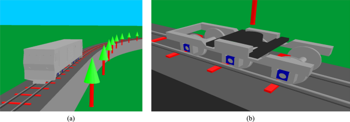
a Perspective of the locomotive running on a realistic track; and b perspective of the bogie frame
3.1 Vehicle model
The vehicle model used in this work is adapted from the model described in detail by Millan et al. [40]. The adaptations are aimed to reduce the computational cost of the simulations and are subsequently used by Pagaimo et al. to demonstrate the application of the flexible multibody methodology employed in this work [39]. The adapted model differs from the original rigid body model by the replacement of the rigid front bogie frame by a deformable bogie frame. The primary suspension is simplified through the removal of the kinematic joints that accurately represent the geometry of the contact between the hornguides of the bogie frame and the axle boxes. Instead, viscous dampers are introduced in parallel with the vertical springs, as well as pairs of horizontal springs between each axle box and the bogie frame to increase the lateral and longitudinal stiffness of the suspension.
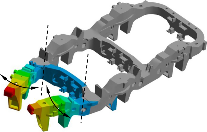
The study of the sensitivity of TDI and MO methods to fatigue cracks requires an initial identification of critical locations in the bogie frame, i.e., the areas where cracks are most likely to initiate and propagate. The bogie frame is modeled in a 3D CAD software and the identification of the critical locations of the bogie frame is performed in a FEM software following the guidelines described in the standard EN 13749 [41], while also prioritizing the welded connections of the bogie frame due to their susceptibility to the propagation of fatigue cracks [8, 42, 43]. Standard EN 13749 establishes requirements and offers examples of static and dynamics tests that can be conducted to evaluate the design of bogie frames. In this work, the test programme for bogies of locomotives under normal service loads resulting from operation running detailed in point F.2.2.2. of annex F is adapted to the configuration of the bogie, considering three axles, and four connection points between the frame and the bolster. The bogie frame model is clamped on the top surface of the middle right horn guide, preventing all the displacements of the nodes of this surface. The bogie frame is simply supported on the top surface of the remaining horn guides, preventing only the vertical displacements of the nodes. The distributions of the von-Mises stresses on the structure are analyzed in three distinct static load scenarios according to section C.4.2. of the standard. The critical locations are the areas of higher stress concentration, when subjected to tension or shear forces that contribute to the propagation of cracks. The identification process is not fully described in this work for the sake of brevity. However, the analysis shows that the most relevant critical location is the welded connection between the front transversal beam and the lateral side frame, highlighted in Fig. 3. After the 3D CAD model is used to identify the critical location using static analysis, it is then modified to incorporate synthetic cracks. Therefore, the task of identification of the critical locations is fully independent from the process of damage localization using the transmissibility-based method, which is the main objective of this work.
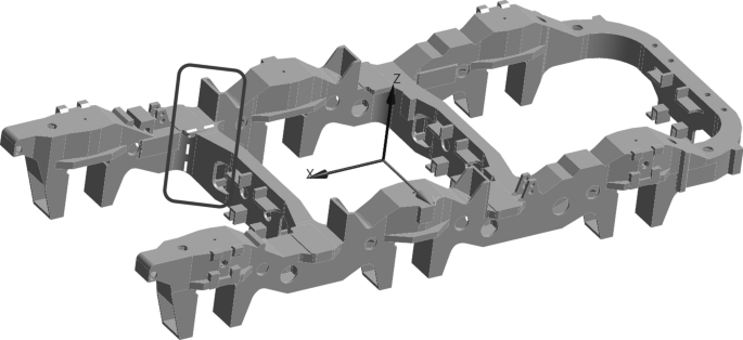
Position of critical location on the bogie frame
The flexible multibody formulation used requires the modal matrix X containing the modes of vibration, and the diagonal matrix with the squares of the natural frequencies Λ. These entities are the outputs of a modal analysis, which involves a linearized bogie frame model, disregarding the physical nonlinearities, such as the normal and friction forces that develop between the contacting surfaces of the crack [44]. The synthetic crack is directly defined in the 3D CAD model, in the vertical cross-section plane that connects the front transversal beam with the right lateral side frame, as shown in Figs. 3 and 4. The external shape of the cross-section is rectangular, approximately 170 by 230 mm, and the average wall thickness is roughly 15 mm. Six scenarios are characterized by different crack area magnitudes: 0%, 20%, 40%, 60%, 80%, and 100% of the area of the cross-section of the welded connection. Each scenario involves a different model of the bogie frame and, consequently, a distinct set of matrices X and Λ. The six models were defined ensuring that the positions of the nodes of the finite elements are the same, and that only the connectivities between nodes are changed, to represent different crack sizes. The bogie frame is described by approximately 45,000 structural 3D 10-node tetrahedral solid finite elements. The FE model was subjected to a mesh convergence procedure—the effect of the reduction of the size of the elements is assessed quantitatively by analyzing the convergence of the matrix of the natural frequencies of the structure Λ, and qualitatively by inspection of the modes of vibration in X. Additionally, the FE mesh was further refined in the vicinity of the crack to increase the accuracy of the deformation results in this area.
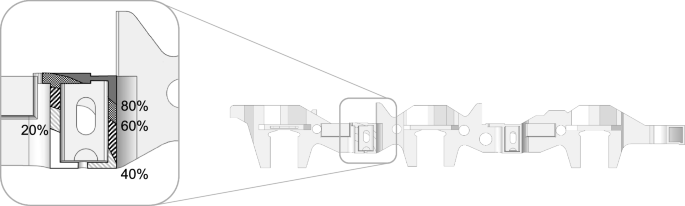
Geometry of the crack plane with the identification of the crack tip position as a function of the damage magnitude
The selection of the modes of vibration considered in the modal matrix is relevant. Minimizing the number of modes allows reducing the number of equations of motion that must be solved, and the number of modal coordinates to be integrated, while maximizing the time step used in the integration scheme. Conversely, the increase of the number of modes improves the accuracy of the description of the deformations. The first 30 flexible modes of vibration, associated with a frequency range of approximately 31.1–377.2 Hz, are deemed a reasonable compromise between these conflicting effects. This set includes modes of vibration that are relevant to describe the lateral movement of the side frame in the vicinity of the crack, such as the 4th flexible mode shape, associated with a natural frequency of 52.2 Hz, depicted in Fig. 5.
Bogie frame deformation associated with the 4th mode of vibration, with a natural frequency of 52.2 Hz – lateral movement of the front ends of the side frames, in phase opposition
3.2 Flexible multibody simulations
The simulations are performed considering the locomotive running at a constant speed of 60 km/h. The locomotive runs on a straight track section with realistic track irregularities that are synthetically generated using a multivariate statistical process [45]. The results of the simulations include the accelerations on the points depicted in Fig. 6, that represent a system of virtual accelerometers distributed along the bogie frame. Nodes 11–16, located in the vicinity of the crack, aim at capturing local effects in the accelerations. Nodes 3–8 are positioned symmetrically with respect to the vertical plane of symmetry of the bogie frame, oriented in the longitudinal direction, and provide a reference that can be used to evaluate asymmetries in the structural dynamics. Nodes 1, 2, 9, and 10 are located on the outer edges with the purpose of capturing global changes in the vibrations. The proposed system of sensors is a first iteration, defined taking into consideration the a-priori identification of the critical location. Certainly, in a real scenario, the sensor system should be further enhanced to cover other critical areas of the bogie frame to improve the sensitivity to damage in distinct locations. Nonetheless, the critical locations must be prioritized.
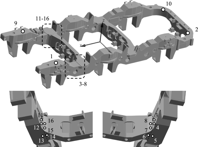
Baseline set of virtual accelerometers
The transmissibilities are computed from the PSDs of the lateral accelerations as described in section “Transmissibility damage indicator”. The PSDs are defined as Welch’s PSD estimates, with a Hamming window of 4 s and 75% overlap. The transmissibility curves τ19 (ω) in Fig. 7 relate the lateral accelerations of sensors 1 and 9, considering the bogie frame in the nominal condition, and damage scenarios of the crack with 20% and 40% of the area of the cross-section area of the transversal beam. Figure 7 shows that a crack with moderate dimension affects the magnitudes and peak-frequencies of the transmissibility curves τ19 (ω), demonstrating that the transmissibilities are sensitive to the synthetic crack. The results also suggest that the lower frequency range of the transmissibility curves, up to approximately 40 Hz, is not affected by the presence of the crack.
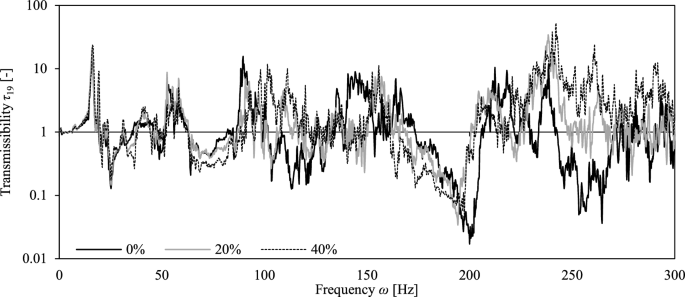
Transmissibility curves of the lateral accelerations measured at points 1 and 9: nominal condition (0%) vs. damage scenarios (20%, 40%)
4 Results damage detection using transmissibility-based methods
This section focuses on the application of the Transmissibility Damage Indicator (TDI) method and the Maximum Occurrences (MO) method with the goal of detecting and locating structural damage of the bogie frame. The transmissibility curves are computed using the lateral accelerations measured in the virtual sensors because in this study they are overall more sensitive to the crack. Nonetheless, in general, the longitudinal or vertical accelerations on the sensors may also be used.
The results presented in this section follow the post-processing of the simulation outputs in the frequency range of 20–150 Hz. The lower limit avoids the frequencies under 20 Hz, that are most commonly associated with the rigid body motion of railway vehicles [46]. Under this value, the effect of damage is assumed negligible, and this assumption is supported by the inspection of Fig. 7. The upper limit of 150 Hz is approximately half of the highest natural frequency included in the set of modes of vibration that are used to describe the structural deformations of the bogie frame. The lower frequencies of the response are the ones most accurately represented by structures whose deformations are modeled as a superposition of modes of vibration.
To compute the TDI and the MO, the sensors shown in Fig. 6 are combined into sets, with sensors in the left and right sides of the bogie frame positioned symmetric relative to a vertical plane oriented along the longitudinal axis of the bogie. All the possible combinations of 4, 6, 8 and 10 sensors out of 16 sensors are evaluated, resulting in a total of symmetric sensor sets.
4.1 Transmissibility damage indicator
4.1.1 Sensitivity of TDI to differences in the track geometry and the time length of signals
Prior to the assessment of the sensitivity of TDI to damage, this subsection focuses on the effect of the differences in the track geometry and the length of the acceleration signals on TDI, for scenarios with the bogie frame in the nominal condition. The TDI method requires the comparison between a reference signal, under nominal condition, and a measured signal, at an unknown condition. If these signals are not recorded under the exact same conditions (speed, track, etc.), the difference between the signals will result in a reduction of the TDI, irrespective of the condition of the vehicle. Therefore, it is essential to evaluate how such changes affect the TDI, to ensure that the TDI has a greater sensitivity to damage than to differences in operating conditions.
Figure 8 presents boxplots of the TDI values, for the 210 symmetric sensor sets, considering three different durations of the acceleration signals: 10, 15, and 20 s. The TDIs are evaluated, for the scenario of nominal condition, with reference and measured signals measured in different track sections, yet have similar statistical properties, i.e., the reference and measured signals are obtained at straight tracks with different irregularity profiles that have similar statistical properties following the multivariate statistical process [45]. The results show that the increase in the time signal to 20 s leads to the narrowest distribution of the values of TDI, as well as the highest median value of TDI, at 0.933. On the contrary, the decrease in the signal duration to 10 s leads to the widest distribution of TDI and the lowest median value, at 0.891. This reduction in TDI shows than the reduction of the signal length results in an increase in the sensitivity to the effect of the discrete differences in the track geometry, despite the condition being nominal. From a practical point of view, the longer the signal, the more difficult to record, store, and post-process the information in a timely manner to issue alerts, if necessary. With a median value of TDI of 0.916, the signal duration of 15 s seems to provide a good compromise between low sensitivity to differences in the track input between track sections and smaller post-processing effort, and will be used in the following subsections.
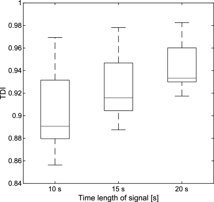
Boxplot of the TDI results, for the 210 symmetric sensor sets, as a function of signal length under nominal conditions of the bogie frame (reference and measured lateral acceleration signals with different lengths and recorded in different track sections)
4.2 Comparison of the sensitivity of TDI to differences in the track geometry and early damage
The assessment of the sensitivity of TDI to the differences in the track geometry, in the previous subsection, is followed by its comparison with the sensitivity to early damage, which is of prime importance. Early detection of the damage is desired to allow inspection and maintenance actions to be developed in a timely manner. Therefore, the values of TDI for a given damage size must be lower than the values obtained for the vehicle in nominal condition, when running in different track sections. Otherwise, there is either the potential for false-positives, or the late warning for inspections or immobilization of the vehicle. In this manuscript, early damage is analyzed through the scenario of a crack of 20% of the area of the cross-section in the critical location.
Figure 9 allows the analysis of the sensitivity, considering reference and measured signals of 15 s length. The results are grouped into 4 subplots, considering sets of 4, 6, 8 and 10 sensors. The markers colored in black are associated with the set identified in the title of the plot, while the markers colored in gray result from all the other sensor sets, to allow for the comparison. The horizontal axis is associated with the value of TDI computed using the different sensor sets evaluated, in the scenario of 20% damage level. The vertical axis shows the TDI resulting from the comparison between signals recorded on the two different sections discussed in the previous subsection, with the bogie in nominal condition. To better explain this, if the sensitivity of a given set of sensors to 20% of damage was the same as it is to the differences in track sections, the abscissa and ordinate of the point would be the same, and the point would lie on top of the diagonal dashed line. Therefore, to effectively detect damage, the points must lie on the left side of the dashed line. Otherwise, the sensitivity to track differences is larger than it is to damage. Overall, the results exhibit a trend where sensors that are more sensitive to early damage are also more sensitive to the differences in the track input for the case of nominal condition. These results support TDI as an apt tool to detect damage for the structure of interest and in the conditions studied. Additionally, the distribution of the markers in Fig. 9 reveals that the results are aggregated into clusters. Further investigation is needed to understand what the driving factors for the distributions in clusters are, although the position of the sensors included in each set is the most likely cause. This analysis is out of the scope of the present manuscript, but future developments on this work should include the employment of data extraction techniques to further process the sensor data and metadata.
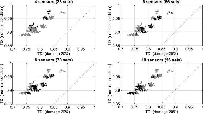
TDI values for the comparison of 20% damage scenario vs nominal condition scenario (reference and measured lateral acceleration signals with a length of 15 s and recorded in different track sections)
4.2.1 Comparison of the sensitivity of TDI to damage progression as a function of the number of sensors
Figure 10 shows the TDI curves as a function of the damage levels, from the nominal condition (0%) to the complete separation of the cross-section at the critical location (100% damage level). The signals have a length of 15 s, and the reference and measured signals are recorded in different track sections, but with the same statistical properties following the multivariate statistical process [45]. The results are grouped into 4 graphs, each one emphasizing the sensor sets with a specific number of sensors. The curves colored in black are associated with the group identified in the subtitle above, while the curves colored in gray are the superposition of the curves from all the other groups of sensor sets, to allow for a global comparison.
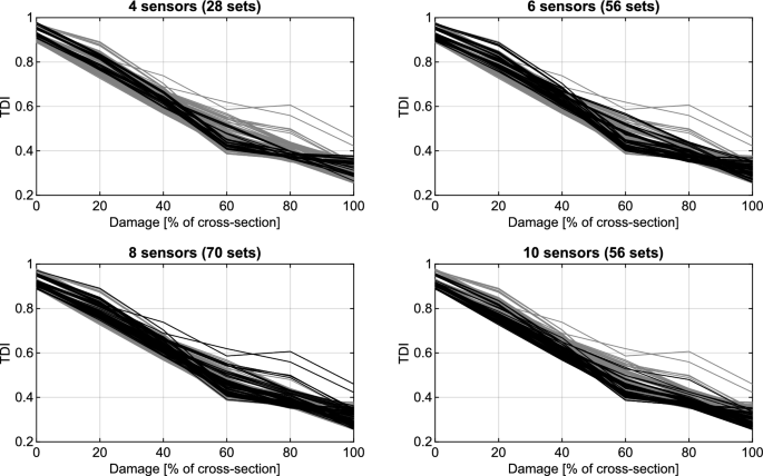
TDI values for different sensor set configurations as a function of the damage level. (reference and measured lateral acceleration signals with a length of 15 s and recorded in different track sections)
In agreement with the results shown in the previous subsections, considering the reference and measured signals are recorded in different track sections, the TDI values for the case of the nominal condition are below one, and are all above the value of 0.88. From the nominal condition to the 20% damage level, the TDI values decrease with different magnitudes, depending on the sensor sets. It is using certain sets of 10 sensors that the TDI presents smaller values. Indeed, the results globally suggest that increasing the number of sensors positively influences the sensitivity of the TDI to damage. The lowest value of TDI for the 20% damage level is 0.726 with the sensor set (1, 2, 3, 4, 6, 9, 10, 11, 12, 14). Above the 20% damage level, with some exceptions, the values of TDI decrease monotonically with the increase in the damage level, down to the range between 0.2 and 0.4, at the 100% damage level. The results show that the number and configuration of the sensor sets have a relevant effect on the sensitivity of the TDI to damage.
4.3 Maximum occurrences
The MO method can be used to estimate the location of the damage, as a complement to TDI. Figure 11 depicts three matrices of MO for a system of 4 sensors, the set (1, 8, 9, 16), which can be seen in Fig. 6. These sensors are on the front end of the bogie frame, two on each side, and sensor 16 is in the vicinity of the crack. Each matrix in Fig. 11 is associated with a different magnitude of crack area and the results are obtained considering the 20–150 Hz frequency range. Each square is associated with a particular pair of sensors, identified by their IDs. The darker is the shade of the square, the higher is the number of occurrences, i.e., the number of frequencies at which the difference between the associated entries of the nominal and damaged condition matrices is maximum. For instance, the matrix on the left shows the sensor pair with the maximum number of occurrences for 20% crack area is (9–16). In this case, there were 252 frequencies at which the differences between the transmissibilities between sensors 9 and 16, for the nominal and 20% damage scenarios, were the highest among all the entries in the condition matrices. Following an inspection of Fig. 6, this sensor pair suggests the front right end of the bogie frame, which corresponds to the area where the synthetic crack is located. The matrix in the middle is associated with the scenario of 40% crack area and shows the sensor pair with the highest number of occurrences is (1–16). Sensor 1 is in the left side of the bogie frame and is not located in the vicinity of the crack, whereas sensor 16 effectively corresponds to the area where the crack is located. The matrix on the right, associated with the scenario of 60% crack area, again indicates the sensor pair (9–16).
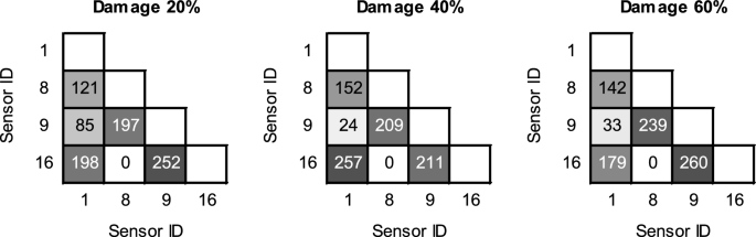
Matrices of Maximum Occurrences (sensor system 1, 8, 9, 16)
Figure 12 shows similar results for the sensor system involving a system of 6 sensors, set (1, 2, 8, 9, 10, 16). This sensor system results from the addition to the previous set of the two sensors located at the rear end of the bogie frame, far from the transversal beam where the crack is located. The sensor pair with the maximum number of occurrences is consistently (9–16). The combined inspection of the results in Figs. 11 and 12 suggests that the increase in the number of sensors may improve the sensitivity of the MO method and enhance the capacity to locate the damage.
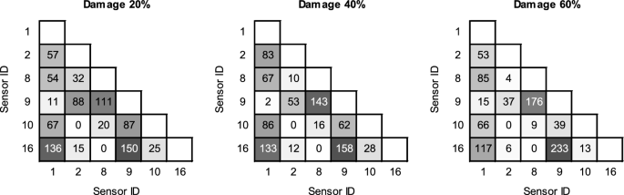
Matrices of Maximum Occurrences (sensor system 1, 2, 8, 9, 10, 16)
5 Conclusions
In this work, the condition assessment of the bogie frame of a locomotive is achieved using the TDI and the MO methods, that are two damage detection methods based on the concept of transmissibility. The results of multibody simulations provide the nominal and abnormal dynamic response of the vehicle running on a track section with realistic track irregularities. In particular, the lateral accelerations measured by a set of virtual sensors distributed on the structure of the bogie frame are the result of a set of simulations of the vehicle–track interaction, considering a synthetic crack in a critical location.
The condition matrices of the reference and measured responses, that are formed by the direct transmissibilities between all the points of the structure, are computed in the frequency range between 20 and 150 Hz and the TDI values are calculated according to a scheme that relates the transmissibilities between all the sensors of each sensor system set, instead of the sequential scheme of the original formulation of TDI. This manuscript includes an analysis on the sensitivity of TDI to the effect of external perturbations. Measurements of longer time signals and over longer track sections allow reducing the variability in the accelerations that is associated with external perturbations, such as discrete differences in the track input. The analysis also shows that the sensitivity of TDI to damage is higher than the sensitivity to the effect of the differences in the track irregularities. Additionally, the results show that the TDI method can successfully detect a crack with a moderate-to-large dimension if the sensor set and the post-processing are adequate.
After the damage detection using the TDI method, the MO method allows the localization of damage through the identification of the entry—in a matrix that combines different pairs of sensors—that presents the largest differences between the nominal and measured transmissibility matrices. The indices of the entry indicate the pair of sensors most sensitive to damage. Overall, the results demonstrate that both transmissibility-based methods are effective to detect and identify damage, provided that the sensor set is satisfactory, the response is measured in predetermined track sections, and the vehicle response is adequately post-processed.
The results of this work suggest further research actions. The application of the transmissibility-based methods in a real operation can benefit from the development of a normalization procedure for the measured signals, which takes into consideration the varying operation conditions, in particular the velocity and the track characteristics. The simulations used to obtain the vehicle dynamic behavior are limited to straight track sections. However, track transitions and curves subject the railway vehicles to different excitations, which may either reveal or conceal the abnormal behavior of the vehicle. Consequently, it is worth investigating the effect of track curvature on the sensitivity of the transmissibility methods.