Article Content
1 Introduction
Integrating control-flow and data aspects to holistically capture the dynamic evolution of processes is a central problem in AI [16], business process management (BPM) [99], and process mining [88].
Multi-perspective models that reflect this interdependency have consequently emerged [32, 53, 75, 99, 103], in turn calling for analysis and mining techniques able to address such different perspectives. When describing case-centric, data-aware processes, every case comes with a data payload that interacts with the process control-flow in three main ways:
- the execution of activities is not only conditioned by the process control-flow, but also by the data payload;
- similarly, executing an activity does not only result in updating the control-flow state of the case, but also its data payload;
- the data payload can be used to express routing data-driven conditions within decision points.
In this article, we consider classical, case-centric processes where every process execution focuses on the evolution of a main object, indeed called case,Footnote1
Among the process modelling formalisms representing the process control-flow explicitly, Data Petri nets (DPNs) [80, 88] substantiate these three aspects in a concise yet expressive formalism where the control-flow backbone of the process is specified using Petri nets, the data payload consists of a set of variables, and the data-process interplay is reflected in read-write logical conditions over variables, attached to net transitions.
At the same time, within the family of declarative approaches implicitly describing the process control-flow through temporal constraints, data-aware extensions of linear-temporal logic over finite traces have emerged [13, 39, 70], providing logical foundations for multi-perspective variants [31, 86, 104] of the Declare declarative process specification paradigm [42, 94]. In this paradigm, formulae combining temporal operators and conditions over data are employed to simultaneously constrain the evolution of cases and the data they carry.
Notably, which data are actually considered – and which corresponding data conditions can be expressed – depends on which datatypes are considered, heavily impacting on the expressiveness of the resulting setting. Variables may in fact carry simple values like strings or numbers (to, e.g., store the delivery address and the cost of an order), or more complex data structures such as vectors or full-fledged relational databases (to, e.g., store the items contained in an order) [14, 34, 54].
These advances in the (formal) representation of processes are in par with an increasing shift in process mining techniques towards data-awareness. This closes a gap existing in process mining: on the one hand, event data have always been intrinsically multi-perspective, as events in a log come with a timestamp, a reference activity, and (optionally) a responsible resource and one or more data attributes [2]; on the other hand, process mining techniques typically focus on a single perspective at a time, in the majority of cases only retaining reference activities and the qualitative temporal ordering of events, without considering data attributes at all.
Besides representational challenges related to modelling data-aware processes, moving to data-aware process analysis and mining poses a central, computational problem: even under the classical assumption that the process control-flow is bounded, the presence of data makes the overall state space of the process infinite, a difficulty that transfers to process analysis and process mining tasks – both in terms of decidability/complexity, as well as when it comes to practical feasibility [83, 90].
To face such computational challenges, an effective strategy is to avoid the development of ad-hoc algorithms, and instead compile analysis and mining tasks into tasks that can be natively addressed using artificial intelligence (AI) techniques. Within the wide container of AI techniques, Satisfiability Modulo Theories (SMT) [19] naturally matches data-awareness. From the modelling point of view, SMT provides a unified framework to describe first-order formulae dealing with different theories, where each theory provides the logical counterpart of a specific datatype (such as real numbers and arrays) together with its domain-specific predicates (e.g., predicates to compare two real numbers or to check the length of an array). From the reasoning point of view, solid technology is available to check satisfiability of such formulae, with highly performing dedicated solvers for specific theories [17, 50, 57]. In addition, several solvers also provide support for optimisation, giving raise to so-called Optimisation Modulo Theories (OMT) [102].
In this article, we review how the SMT/OMT paradigm is being effectively exploited to address process mining for data-aware processes. We provide references to corresponding pointers to the technical literature, under an integrated lens.
The article is organised as follows. In Sect. 2, we provide the essential preliminaries regarding SMT/OMT solving. In Sect. 3, we recall case-centric logs and discuss how the data attributes associated to events can be interpreted. In Sects. 4 and 5 we provide a gentle introduction to DPNs and data-aware linear-time logics on finite traces. Section 6 presents the major contribution of this paper, providing a coherent framework where different data-aware process mining tasks, paired with dedicated process analysis tasks, are integrated to tackle data-aware process mining. We conclude by outlooking open challenges.
2 Satisfiability Modulo Theories
When formalising systems in logic, it is often necessary to express formulae involving not only boolean variables, but also variables referring to numbers or more complex data structures such as relations, uninterpreted functions, arrays, bit-vectors. This, in turn, calls for combined reasoning on the theories underlying these different datatypes. In this respect, Satisfiability Modulo Theories (SMT) [20] extends propositional satisfiability (SAT) to satisfiability of first-order formulae with respect to combinations of background theories. SMT solvers extend SAT solvers with specific decision procedures customised for the specific theories involved in the formula of interest. SMT solvers are useful both for computer-aided verification, to prove the correctness of software programs against some property of interest, and for synthesis, to generate candidate program fragments.
Well-studied SMT theories are the theory of uninterpreted functions , the theory of bitvectors and the theory of arrays . SMT solvers also support different types of arithmetics for which specific decision procedures are available, like linear arithmetics ( for integers and for rationals). Notable examples of widely adopted SMT solvers are Yices [4, 57], Z3 [51, 93], CVC5 [1, 17], and MathSAT5 [3, 43]. SMT-LIB [18] is an international initiative with the aims of providing an extensive on-line library of benchmarks and of promoting the adoption of common languages and interfaces for SMT solvers.
All in all, SMT solving relies on a universal, flexible and largely expressive approach that allows us to exploit a full-fledged declarative framework, where the actual computations are discharged to very competitive SMT solvers.
Finally, it is important to point out that many SMT solvers are also equipped with optimisation functionalities, tailored to solve problems based on Optimisation Modulo Theories (OMT) [101, 102]. OMT extends SMT by singling out, among the different satisfying assignments for the formula of interest, those that are optimal with respect to a given objective function.
3 Data-Aware Logs and Traces
We are interested in process mining over data-aware traces, that is, traces where the data payload carried by events is taken into consideration when solving process analysis and mining tasks. Our focus is on conventional case-centric process mining, where a (data-aware) event log is a set of traces denoting the evolution of cases through the process, each trace is a sequence of events, and each event comes with a data payload that is considered as a first-class citizen in the analysis.
Notably, this in line with the conventional definition of event log [5], and also with the XES standard for representing event logs [2].
More in detail, we assume that the data payload of each event in a trace refers to the values that a set V of case variables take upon the occurrence of that event. Each variable in is typed, and each type comes with a (typically infinite) data domain , as well as with domain-specific predicates expressing conditions on the values that such a variable can take within its domain. For example:
- a rational variable may be subject to comparison conditions, or in a richer setting, also to arithmetic conditions;
- a variable pointing to a relation may be subject to database operations for inserting/removing/modifying tuples of that relation.
In this light, we define a trace more abstractly than in classical definitions [5].
Definition 1
(Event, trace) Let be a set of variables. An event e over is a set of assignments, one per variable in , mapping that variable to a corresponding value in its domain: – where we write to indicate that in e. A trace over is a finite set of events over .
The following observations are important:
- 1.It is customary to define a dedicate variable for timestamps. This is done by assuming that, among the available datatypes, there is one datatype for timestamps, which can be substantiated using different concrete datatypes (such as, integer), with the only requirement that is equipped with a comparison operator to check whether an event comes before another event.
- 2.If a timestamp variable is employed (say, variable with , it is possible to directly reconstruct how events are sequenced in a trace, by comparing two events through the comparison over their timestamps. Specifically, we can see a trace as a sequence by introducing an ordering such that for every , we have if and only if .
- 3.Activity names, transactional lifecycle indicators, as well as resources, can all be captured through dedicated variables; this is, again, in line with XES, where all these aspects are captured as extensions of a core representation consisting only of events and their sequencing.
- 4.The representation of Definition 1 is general enough to accommodate settings that differ in their logging strategy. For example, if an event does not declare the value of one of the variables, one may assume that, by law of inertia, that value corresponds to that of the previous event (and so, in our representation, the assignment should simply be copied). At the same time, we stress the importance of explicitly pointing out these assumptions, as otherwise the same event log could lead to different interpretations.
Notice that while we follow a case-centric approach, the fact that variables may come with a complex datatype (such as a relation or other types of data structures) makes it quite general, and able to directly accommodate approaches that go beyond XES and tackle events operating over multiple objects. We comment on these so-called object-centric logs in Sect. 7.
4 Data Petri Nets
A process modelling language whose executions naturally match the notion of data-aware trace discussed in Sect. 3 is that of Petri nets with data (DPNs) [80, 88]. We provide a gentle overview of this approach, covering the model, its execution traces, and its execution semantics.
4.1 The DPN Model
A DPN is a Petri net equipped with two additional components:
- 1.a finite set of case variables, conforming to what described before;
- 2.a decoration of the net transitions with constraints that read such variables to express data guards, and that write such variables to express controlled updates – to enable this, constraints are expressed as formulae containing conditions over variables in , mentioned in read or write mode (using r and w as variable superscript, respectively). These formulae can be constrained by several first-order theories, such as linear arithmetic, EUF, relational theories [60].
Figure 1a shows a DPN that models a simple auction process. Every auction represents a case, equipped with two variables: , with variable o holding the last offer, and t a timer. Constraint associated with action expresses that a bid can be placed only if the current value of t is positive, and that when executed, it will increase the value of o.
The atomic conditions used within constraints depend on the datatypes of the variables, and on the available predicates. In the auction example, both variables maintain rational values, subject to linear arithmetic conditions. However, more restricted settings may suffice, like those recalled next:
- monotonicity constraints (MCs) admit only variable-to-variable/constant comparisons wrt. , <, , for variables with domain or , such as or ;
- integer periodicity constraints (IPCs) have the form , for , , or , for variables x, y with domain and ;
- gap-order constraints (GCs) have the form for x, y integer variables or constants, and .
4.2 Executing a DPN
To track the evolution of a case through the process, one needs to recall at once the control-flow state of the net, together with the current values assigned to the case variables. Formally, a state in a DPN is a pair of a marking M and an assignment that maps V to values (according to the datatype associated to each variable). We fix some initial assignment, and call a run a finite sequence of transition firings in the underlying Petri net that respect guards. For instance, a possible run for the DPN in Fig. 1 is
It is easy to see how a DPN run relates to the notion of data-aware trace as of Sect. 3: one just selects the assignments from each state of the run. Logging the name of the last executed activity, which is essential in process mining, can be done by introducing a dedicated case variable a of type string, ensuring that whenever a transition fires, a gets updated with the name of the executed activity. For example, the guard associated to in Fig. 1 can be modified according to this principle by inserting a third conjunct of the form . Furthermore, a surrogate, start event can be inserted to keep track of the initial values for the case variables. With this notions in place, the run above would yield the following trace:
The timestamps of executed activities can be tracked by introducing a dedicated, rational case variable ts in the DPN, ensuring that whenever a transition fires, that variable is written to a value strictly greater than the one it currently maintains (so as to respect the flow of time). This is done through an atomic guard of the form .
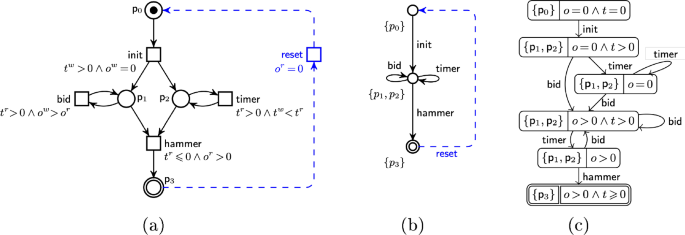
Example of a DPN (a), together with its corresponding DDS (b) and constraint graph (c) (from [96])
4.3 From DPNs to DMTs
For process analysis and mining tasks, it is customary to deal with a different formal model of the process, which directly results from the input DPN, under the assumption that concurrency is interpreted by interleaving. This leads to so-called data-aware dynamic systems (DDSs) [81], which are labeled transition systems where transitions are associated with constraints as above.
Although recently the need of more sophisticated data types and first-order theories has emerged in process science [60, 75], classical DDSs only support linear arithmetical theories, drastically limiting their expressiveness and their applicability in real BPM scenarios [34, 35]. For this reason, data-aware processes modulo theories (DMTs) have been introduced in [76, 77]: they are general dynamic systems manipulating variables that can store arbitrary types of data, ranging over infinite domains and equipped with domain-specific predicates. DMTs strictly generalize DDSs to support arbitrary first-order theories (in the SMT sense). Although they are intrinsically infinite-state systems whose states are characterized by the content of their global variables, DMTs can be enriched with finitely many explicit control states, as illustrated in Ex. 3 in [77].
Notably, every bounded DPN induces a corresponding DMT , straightforwardly defined by considering that each one of the (finitely many) reachable markings in the DPN becomes a control state in the DMT. Figure 1b shows the auction process as a DMT – this specific case only presents arithmetical conditions, so we directly formalize it as a DDS.
4.4 Execution Semantics and Symbolic Representation
The execution semantics of a DMT is an infinite-state transition system, where each state holds the current control-flow configuration (a marking in the DPN case, or the control state in the DMT/DDS case), together with the current assignments of the case variables. Infinity here arises due to the presence of infinitely many distinct assignments for case variables with infinite data domains. In Fig. 1, for example, offers range over all non-negative rational numbers.
To solve analysis and mining tasks with DPNs, it becomes crucial to aim at obtaining finite representations of the infinite-state space (in line with, e.g., [14, 36, 54]) – which cannot be done in general, but can be achieved for certain theories, possibly under suitable restrictions on how the process operates over data variables. A natural way of attacking this problem is by aiming at symbolic representations of the state space, where SMT formulae are used to represent (possibly infinitely many) distinct states that behave equivalently in the context of the process execution. This idea is at the basis of a long series of results in the (symbolic) verification of infinite-state systems. In the context of process science and data-aware processes, such results are surveyed in [75].
When dealing with DMTs, this technique is substantiated through so-called constraint graphs. These are semi-symbolic representations of the state space induced by the input system, where each state contains a reference to the corresponding control state of the DMT, and a formula constraining which assignments are accepted for that state. This has been initially defined for the specific case of DPNs/DDS with monotonicity constraints [62, 81], then extended to other cases in [66], and finally it can be generalised to richer theories (as in the case of DMTs [77]).
The main idea underlying the constraint graph construction is to traverse the DMT in a forward fashion. While doing so, constraints are accumulated, taking into account the peculiarities of read and write guards, and inserting inertial constraints indicating that untouched variables maintain their value. In this respect, a symbolic state is a control state decorated with a formula for the accumulated constraints, which characterises the set of assignments leading there. Importantly, the same control state may now appear multiple times. Moreover, the construction is in general infinite, though for expressive and relevant classes of processes, finite constraint graphs can be obtained.
At every step, one starts from a symbolic state s, and symbolically fires a transition to get a new candidate symbolic state . SMT solving is then applied for a twofold reason. First, it is used to check whether the formula of is satisfiable: only in that case, is indeed a reachable state, and should be considered as part of the constraint graph. Second, in order to prune the state space, the SMT solver can optionally be used to check whether is genuinely new, or a semantically equivalent state has already been inserted in the constraint graph. In the former case, is added to the constraint graph, together with a labelled transition linking s to ; otherwise, if an equivalent exists, then is discarded, and s is linked to . However, the second check is feasible only when it is possible to handle in some form the quantifiers involved in formulae [37, 66, 74].
Figure 1c shows the constraint graph of the auction DPN.
Importantly, the constraint graph should be interpreted existentially, that is, when there is a path in the constraint graph, it means that the corresponding sequence of transitions can be executed for some sequence of variable assignments satisfying the respective state formulae. Consider, for example, the auction process in Fig. 1. The symbolic state can be reached with any possible value for variable t, but only with a positive value for t it is possible to apply the transition therein.
We comment on the finiteness of the constraint graph, and the impact on reasoning over DPNs, in Sect. 6.2.
5 Data-Aware
(linear-time logic on finite traces [48]) is one of the most widely employed temporal logics to express properties and constraints of finite-length traces.
Traditionally, temporal logics are used to express (un)desired properties of a dynamic system, while the system itself is specified using a different formalism. For example, one may use to verify properties of (finite traces of) a Petri net. A less conventional approach is to declaratively describe the dynamic system itself using temporal logics. Within process science, has seen wide employment in this second acceptation, to provide a formal semantics for declarative process modelling approaches, most prominently Declare [42, 94]. The main idea is to implicitly describe the process control-flow through a declarative specification that consists of a set of temporal constraints, so that a trace belongs/conforms to the specification if and only if it satisfies all the constraints contained in the specification.
No matter which of the two usages is adopted, expressing properties and constraints of data-aware traces (as of Sect. 3) calls for
- 1.linear temporal operators to relate different positions (or instances) of the trace;
- 2.local data conditions to inspect and express properties of the assignments contained in the trace;
- 3.data conditions relating different assignments over time.
These three features are present in first-order variants of , which have been studied either in the classical setting of a single infinite interpretation domain where constants can be compared with (in)equality [13, 39], or the “modulo-theory” setting where multiple datatypes are considered [70]. We provide a bird-eye-view of the latter setting, considering a simplified variant of the logic in [70, 71]. This variant, called , has been originally introduced in its full generality in [77],Footnote2 and exactly mirrors the notion of trace defined in Sect. 3.
Definition 2
(Syntax of ) Let be a set of variables. A formula over is defined according to the following syntax
where q is a condition over , possibly mentioning primed versions of variables therein (i.e., versions such as and for ), and constants in the data domains of the types of variables in V.
Formulae of are interpreted in an instance of a trace as per Definition 1. In the definition:
- and are the next and (strong) until temporal operators, used to move over consequent instants of the trace. Specifically φ indicates that the next instant of the trace exists, and holds therein; φ indicates that holds in a future instant k of the trace, and holds in every instant between the current instant (included) and k (excluded).
- Conditions only mentioning non-primed variables (i.e., variables from ) are local conditions checked on the current instant of the trace;
- Conditions mentioning primed versions of variables express data conditions over different instants. Specifically, a variable with n primings denotes a lookahead variable that refers to the value the variable holds n instants after the current one. In this respect, x refers to variable x in the current instant, while has a lookahead of 3, and refers to x three instants after the current one. This can be used to express conditions that relate different assignments over time. For example, condition expresses that the value of x will increase in the next instant, and will then remain constant in the consequent instant.
Importantly, (like the richer logic ) can only relate variables from instants that are at a bounded distance to each other – the maximum distance being implicitly determined by the largest employed lookahead. This enforces a well-behaved nesting of data conditions within temporal operators [70]. Relaxing such a nesting, which is needed to capture conditions relating variables in arbitrarily distant instants, causes basic reasoning tasks to become highly undecidable, even in the very restricted setting where variables range on an infinite domain whose elements can only be compared by (in)equality [39, 52].
Consider a process operating over two rational variables x and y. The following formula (without lookahead)
expresses that y is non-negative until the trace reaches an instant from which x is always greater than y.
The following formula with lookahead
captures that x is strictly increasing (formulated by expressing that it is always the case that the next value of x is greater than the current one), and at some point holds value 2.
As described above, can be used:
- to express properties of (the runs induced by) a DPN, relying on the compatibility between data-aware traces and DPN runs (cf. Sect. 3);
- to declaratively specify a data-aware process as a set of temporal constraints.
In the latter setting, provides logical underpinnings for data-aware extensions of Declare [31, 86, 95, 104]. Binary Declare templates like, for example, the response template (indicating that whenever a source activity A occurs, then a target activity B will occur later), are usually lifted to a data-aware setting by enriching the template with:
- a source condition associated to A;
- a target condition associated to B;
- a correlation condition relating the payload of A with that of B.
Intuitively, in the case of response the meaning of the constraint becomes: for every instant i, if A occurs in i and is true in i, then there must be a later instant such that B occurs in j, is true in j, and is true once evaluated over i for A’s variables, and j for B’s ones. The case of chain response is handled analogously, with the only difference that .
With this approach, one can ground the response template (respectively, the chain response template) to express, for example, that whenever an order is paid by a person with credit card as payment mode, then a receipt must be later (respectively, immediately next) issued to that same person.
Considering the bounded lookahead property of discussed above, we have that naturally supports the formalisation of Declare templates with source and target conditions, and covers correlation conditions relating positions with a bounded lookahead. In the order example above, the response version cannot be captured in , while the chain response version can be captured as follows:
assuming that a, m, and p are string variables respectively denoting activities, payment modes, and persons.
As we will see later in Sect. 6, while the bounded lookahead property is essential in the context of reasoning, it can be lifted when dealing with discovery and conformance checking. Intuitively, this is due to the essential fact that in these tasks there is always a maximum bound on the length of traces to be considered (in discovery, determined by the analysed log, and in conformance checking, by the analysed log and the considered specification).
6 Data-Aware Process Mining Tasks
We are now ready to discuss how the languages and techniques described so far have been employed to solve key data-aware process mining tasks, using SMT/OMT solvers as the core, underlying algorithmic technology.
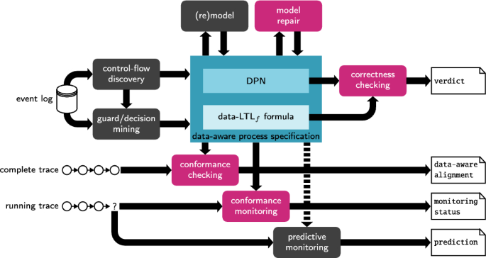
Overall schema showing key data-aware process mining tasks. SMT-based tasks are shown in magenta
Figure 2 takes the standard schema describing a process mining framework, in particular the version shown in [6], and adapts and refines it to the setting of data-aware traces and data-aware specifications – formalised using DPNs or . Among the shown tasks, in magenta we report those mainly tackled with SMT in the state of the art.
We next comment each task in more detail, providing references to the literature.
6.1 Discovery with Loosely-Integrated Techniques
Discovery of data-aware process specifications has been tackled so far through a loosely integrated approach that, in its essence operates as follows.
- 1.a pure control-flow specification is discovered using conventional techniques – for example, producing a Petri net or a Declare/ specification;
- 2.elements that are conditioned by data are identified within those specifications – for example, singling out choice points and activities in a Petri net, or activities in a declarative specification;
- 3.data attributes corresponding to such elements are extracted, and a decision mining task is cast on them;
- 4.the result of decision mining is, per element, integrated into the control-flow specification, yielding a final, data-aware refinement of it.
This approach has been applied to discover DPNs, where decision mining is used to attach read guards to transitions [88, 89], and to discover data-aware Declare specifications, using decision mining first to mine source and target conditions [86], and in subsequent work also addressing correlation conditions [79].
A strong point of this approach is that existing techniques separately dealing with control-flow and decision mining can be seamlessly integrated.
A downside is that there is no guarantee that the combination of the two dimensions – discovered separately and integrated a-posteriori – suitably works. In particular, it has been shown that this form of discovery may produce unsound DPNs – a phenomenon that can also arise when a (sound) discovered DPN is later subject to manual re-modelling [67, 68].
This motivates the insertion of two model-driven analysis tasks within a data-aware process mining pipeline:
- correctness checking – to verify whether the (executions of the) DPN satisfy properties of interest, in this case using to formalise such properties;
- model repair – to turn an unsound DPN, or an inconsistent specification, into a sound/correct one, by introducing minimal changes to the original specification.
6.2 Correctness Checking
Checking correctness of DPNs against full has been addressed considering linear-time properties in [77]. In the specific setting of arithmetic datatypes, verification has been tackled studying linear-time [66], branching-time [65], and data-aware soundness [67] properties. It is worth noting that, when analysing DPNs, it is irrelevant whether or not the logic supports lookahead. Intuitively, this is because the DPN itself can impose transition constraints that relate variables across time.
Considering the auction example of Fig. 1, there are two main correctness issues. First, the transition is dead, as whenever marking is reached, then variable o must hold a strictly positive value (as witnessed in the bottom symbolic state of the constraint graph). Second, if after executing transition is fired, writing a value for t that is , then can never fire: it requires , but only lower values of t can be written by further firings of . This, in turn, indicates that variable o will always keep value 0, making it impossible to fire and reach the desired marking .
6.2.1 Linear-Time Properties
In [66], linear-time correctness checking of (the finite runs generated by) a DPN is addressed for formulae over arithmetic datatypes in an existential way, that is, verifying whether the DPN can produce some run satisfying the given property.
The approach in [66] lifts to an arithmetic setting the classical automata-based model checking approach for linear-time logics [15]: the formula is encoded into an automaton, which is then combined with the transition system under scrutiny to obtain a cross-product that is inspected for non-emptiness to ascertain whether the property holds. Three challenges arise, though:
- 1.when constructing the automaton of the formula, one has to consider that edges are not propositions, but instead constraints over the theories mentioned in the formula;
- 2.also the cross-product of the formula and of the DPN constraint graph must take into account the fact that edges of the automaton, and symbolic states of the constraint graphs, contain formulae, not mere propositions;
- 3.in contrast to the propositional setting, the cross-product must as we have discussed in Sect. 4.4, even when the transition system of the input DDS is represented symbolically through a constraint graph, it may contain infinitely many states.
The first challenge is tackled, at first, by dealing with constraints at a purely syntactic level. Specifically, they are treated as propositions when building the automaton of the formula – which is then constructed following the standard approach for propositional [46, 48]. The resulting automaton has constraints on its edges. In a second phase, the meaning of constraints is taken into account, to only retain edges whose formulae admit satisfying assignments: SMT solving is employed to only retain edges with satisfiable formulae.
The second challenge is handled similarly: when combining the automaton of the formula with the constraint graph of the DPN, SMT solving is used to decide which states/transitions should be kept, and which should instead filtered out.
The third challenge cannot be solved in the general case, as the correctness checking task is highly undecidable. For example, it is undecidable when employing only a single numeric datatype equipped with increment, decrement, and test for zero [66]. To single out decidable cases, [66] brings forward a semantic property of the input system, called finite history, which guarantees that the constraint graph has finitely many states, in turn yielding a correct and terminating technique for correctness checking. Having a finite history is a semantic property, undecidable to check on its own.
However, it is instrumental to single out concrete settings, defined based on syntactic conditions on the shape of constraints and/or the control-flow structure of the systems, which enjoy finite history, and in turn yield decidable cases. In fact, this approach has been used to reconstruct and generalise decidable cases known from the literature. In particular, [66] identifies the following, well-behaved classes:
- DPNs with monotonicity constraints;
- DPNs with integer periodicity constraints;
- DPNs with gap-order constraints;
- DPNs with unrestricted arithmetics, but used in a controlled way, in particular ensuring that the value of each variable depends only on boundedly many arithmetic manipulations;Footnote3
- DPNs that structurally integrate components falling in two or more of the previous cases.
An important generalisation of such classes has been then achieved in [76, 77], where decidability of correctness checking is obtained for DMTs as well, in case of very general datatypes obeying to mild, model-theoretic assumptions.
6.2.2 Branching-Time Properties and Soundness
When properties are verified on a DPN, it becomes also relevant to inspect the branching structure of the modelled process. This is studied in [65], which introduces a CTL version of restricted to arithmetic datatypes. Among the classes recalled above, decidability is shown to only hold for monotonicity and integer periodicity constraints [65].
Notably, the capability of CTL of mixing linear- and branching-time operators makes it possible to use it to specify a data-aware variant of the well-studied notion of soundness for Petri nets [9], now carried over DPNs. This has been initially introduced in [49, 63] to formally characterise soundness of control-flow processes equipped with (DMN) decisions [21], and then generalised in [67] to the case of DPN with arithmetics.
6.3 Model Repair
As discussed in the previous section, a discovered DPN (possibly subject to consequent manual intervention) may exhibit undesired behaviours. For example, the auction DPN of Fig. 1 is unsound. Unsoundness can be experienced when discovering DPNs using loosely-integrated techniques for the control-flow and data part. Some unsound DPNs from the literature are discussed in [68]. Similar issues may be experienced in the declarative setting, where discovering constraints that are only satisfied by a fraction of log traces may contradict each other, leading to an overall inconsistent specification [41].
Instead of simply rejecting the faulty specification, one may attempt at repairing it, that is, transforming it into a “correct” version, obtained from the original one through a minimal set of changes. In the case of an unsound DPN, that would require to apply minimal changes to it so as to make it sound. In the case of an inconsistent declarative specification, one may identify minimal unsatisfiable cores (that is, minimal sets of constraints causing inconsistency) [44, 87, 100], and then weaken or remove them.
A first challenge is actually to define what minimal set of changes actually means. In fact, one may consider changes at the representation or behavioural level. The first setting considers the effect of changes over the specification itself, such as how many guards are modified when repairing a DPN, or how many constraints are weakened/removed in a Declare specification. The second setting treats the specification as a compact representation of a set of traces, and thus minimality may consider which behaviours are lost/gained when altering the specification. For example, in the case of a DPN, one may consider how many traces disappear, and how many transition firings ending up in a dead state get unblocked upon repairing it.
Model repairs in a data-aware setting have so far being studied only to turn unsound DPNs into sound ones, while to the best of our knowledge no repair strategies have been studied for . More in detail, minimal repairs for unsound DPNs are studied in [108] at the representation level, and in [68] at the behavioural level. Indeed [108] treats the DPN as a (graphical) representation, and minimality considers how many different guards are altered in the repair, and how. In [68], it is assumed that the control-flow of the DPN (stripping off all the constraints) is sound, and that two types of operations can be done in a repair: removal of dead transitions, or modification of constraints, by either relaxing or tightening them. SMT solving and configuration graphs are used to define minimal overall repairs through extension or restriction, measured in terms of removed/newly inserted traces.
Repair by restriction of the auction example leads to two main changes to the DPN in Fig. 1a:
- The dead transition is removed.
- The dead state arising when fires before any firing of , writing a value for t that is 0 or negative, is curated by tightening the guard attached to into . This new guard adds a third conjunct ensuring that either a bid has been placed (thus making ) – and so can fire, or that the written time is positive (thus leaving enabled). As shown in [68], this modification ensures that all the runs accepted by the original DPN are still accepted by the new one, and that the (partial) runs getting stuck in the dead state described above are now able to progress until the final marking – thus guaranteeing minimality.
6.4 Conformance Checking
Conformance checking in a data-aware setting compares logged traces and model traces (that is, traces conforming to a reference process specification) by considering both the sequencing of events and the payloads they carry. In a nutshell, the conformance checking problem takes as input a log/a trace and a process model, and computes various artifacts linking observed and modeled behaviors. Such artifacts are then used for deviation detection, (process model) quality metrics computation, and the like.
6.4.1 Alignment-Based Conformance Checking
A widely adopted conformance checking artifact for a given log trace is that of alignment, indicating how the log trace relates to the closest model trace(s), and computing a related cost [10, 28]. An alignment is a finite sequence of moves (event-firing pairs) s.t. each (e, f) is (i) a log move, if and ( is a symbol denoting skipping); (ii) a model move, if and f is a valid transition firing; (iii) a synchronous move otherwise. Given a log trace and a process model, a corresponding alignment is computed by finding a complete process run that is “the best” among all those the process model can generate. This is done by searching for an optimal alignment using a specific cost function, which can be realised as a distance between two finite strings [10, 28]. In case of logs with uncertainties, one looks into alignments obtained for realisations – possible sequentialisations of (a subset of the) events with uncertainty in a given trace so that timestamp uncertainties are resolved [59].
6.4.2 Alignments for DPNs using SMT/OMT
Checking conformance of data-aware traces to DPNs has been initially tackled in [91], defining and computing multi-perspective alignments for DPNs. Intuitively, mismatches between events of a log trace and corresponding transition firings of the DPN may be caused not only when the reference activities are different, but also in case the data disagree.
Better algorithmic bounds and a more general technique based on SMT/OMT have been then proposed in the conformance-checking approach CoCoMoT [58, 60]. The idea behind CoCoMoT stems from SAT-based approaches for the computation of pure control-flow alignments [27], lifting them to the data-aware case.
This is done in a modular way as follows, under the assumption that the input DPN supports at least one run (i.e., in technical terms, is relaxed data sound). The main modules of the encoding are: (i) the executable process model (EPM) module, which realizes the execution semantics of the input DPN by symbolically encoding all possible valid process runs; (ii) the log trace (LT) module, which accounts for the trace realization in case it contains any uncertainties; (iii) the conformance artifacts (CA) module, which accounts for a conformance artifact of interest as well as for its related decision/optimization problem, i.e., the task that needs to be solved (or decided) in order to compute such artifact.
Each module (with the exception of the part of CA related to the decision problem) is represented as a conjunction of SMT constraints. It is important to stress that the EPM is module symbolically encodes all runs of the DPN up to a given upper bound in length. This is, however, without loss of generality, as for a given log trace, one can compute an upper bound on the cost of the worst possible alignment [58, 60].
The LT module naturally encodes all the aforementioned uncertainties (if any) and, in case of the uncertainty on timestamps, for related events it provides an additional encoding to find a suitable ordering for them.
All the SMT constraints are then put into one conjunction, which is passed as input to an SMT solver in order to solve the associated decision problem. For the case of alignments, CA encodes a selected distance-based cost function defined as the sum of contributions that only depend on the local discrepancies in the moves of the considered alignment (i.e., inductively), and this is done using a finite set of variables that are later used to extract the optimal alignment solution. However, since there are in principle many possible satisfiable solutions, in order to find the best/optimal one, we solve an OMT problem for which a satisfying assignment to all the variables in the encoding is so that the total cost (represented as a single variable carrying the final result of the aforementioned inductive cost encoding) is minimal. This allows us to find a model run which is the closest one to the trace.
In the same manner, one can adjust CA by changing the decision problem associated to the specific conformance artifact of interest. Along this line, [60] brings forward encoding modifications to account for multi- and anti-alignments [26, 40]. To capture different results while computing conformance artifacts, one can also modify CA to account for different cost functions. For example, in [59] it is shown that one can employ a generic cost function whose components can be flexibly instantiated to homogeneously account for a variety of concrete situations where uncertainty come into play.
6.4.3 Dealing with Uncertainty
The approach in [58, 60] has been further extended in [59, 61], dealing with different forms of uncertainty in the input event log, building on [97] and lifting the setting of [69] to the data-aware case. In this extended approach, given a set A of activity labels and a set of attributes names Y, an event is a tuple , where , is a (partial) payload function associating values to attributes from Y, is a confidence that the event actually happened, is a set of activities with related confidence values, and is a finite set of elements from (or an interval over) a totally ordered set of timestamps. The last three values support the following forms of uncertainty: (i) uncertain events, which come with confidence values describing how certain we are about the fact that recorded events actually happened during the process execution; (ii) uncertain timestamps that are either coarse or come as intervals, which in turn affect the ordering of the events in the log; (iii) uncertain activities that in bundle (together with corresponding confidence values) are assigned to a concrete event when we are not certain which of the activities actually caused it; (iv) uncertain data values which, for an attribute, come as a set or an interval of possible values.
6.4.4 Alignments for Specifications
Conformance checking for data-aware declarative specifications has been often tackled following the seminal approach in [31], which focuses on data-aware variants of Declare, and defines conformance through metrics that count how many times a trace “activates” a constraint of interest, and how many times an activation corresponds to a consequent “satisfying target”. Data-aware alignments have been tackled only in [23], considering the fragment of formulae restricted to arithmetical datatypes and to variable-to-constant comparison conditions only. The approach builds on the automated planning-based alignment technique for from [47], dealing with variable-to-constant conditions through an explicit data abstraction technique that propositionalises them in a faithful way. SMT/OMT techniques provide a natural candidate to generalise this approach to richer datatypes and conditions.
6.5 Monitoring Tasks
The general framework in [6] does not only put emphasis on standard, post-mortem process mining tasks conducted on event logs of already concluded process executions. It also includes online tasks of operational decision support, whose goal is to obtain insights on ongoing executions, in turn providing the basis for taking informed countermeasures. While [6] includes predictive process monitoring as an exemplar operational support task, we also include here conformance monitoring, as it naturally connects to the already discussed task of conformance checking, and has been effectively attacked using SMT.
6.5.1 Conformance Monitoring
Conformance checking of declarative process specifications has been extensively studied not only on already completed traces, but also to monitor ongoing executions [85]. In this setting, we speak of conformance monitoring, a task that consists in ascertaining whether the ongoing execution satisfies or violates a given set of temporal constraints.
Interestingly, when such constraints are formalised in , one can deal with a more sophisticated version of this task, known under the name of anticipatory monitoring [82]. The idea of anticipatory monitoring is to verify whether a running trace satisfies a formula, also considering the fact that the trace can continue in any possible way (as we do not yet know what will be its future unfolding). In the field of runtime verification, this led to the definition of different runtime semantics for temporal logics over infinite traces [82], most notably the RV-LTL approach [22], which, given a trace and a formula, refines the two possible outcomes of satisfaction or violation into four possible truth values. Specifically, the verdict of the monitor of a property at each point in time is one of four possible values: currently satisfied (the formula is satisfied now but may be violated in a future continuation), permanently satisfied (the formula is satisfied now and will necessarily stay so), and the two complementary values of permanent and current violation. This immediately shows that monitoring is as hard as checking satisfiability and validity in the logic of interest.
Anticipatory monitoring has been extensively applied in the context of conformance monitoring of Declare/ [42], exploiting the key advantage that, over finite traces, monitoring is well-defined for every linear temporal formula [46]. This is different from the infinite trace-setting, where there are non-monitorable formulae. In addition, anticipatory monitoring of can be operationalised in a very elegant way:
- first, one construct the (deterministic) automaton recognising the language of the input formula;
- second, every automaton state is assigned to one of the four truth values, depending on whether the state is final or not, and on whether it can reach a non-final or a final state.
In [64], this approach has been lifted to the fragment of that restricts to runs over arithmetic datatypes. To handle this much more convoluted case, [64] extends the construction of monitors to suitably address the arithmetic data conditions contained in the formula of interest. The starting point is the automata construction technique used for correctness checking, as recalled in 6.2. However, that technique is not enough: for existential verification problems over DPNs, the automaton of the formula need not to capture all and only those traces satisfying the formula, while a weaker approximation of this set is enough [76, 81].
Such a weaker approximation is instead not fine-grained enough for anticipatory monitoring, where language-preserving automata are needed. [64] tackles this open problem by first considering formulae without lookahead. In that case, a very similar approach to that used in linear-time verification (cf. Sect. 6.2) can be pursued, yielding solvability of monitoring for all arithmetic theories that have decidable satisfiability. As for properties with lookahead, the situation is more challenging, and incurs in even more severe undecidability boundaries than the case of linear-time verification: monitoring solvability is shown to hold for all the cases mentioned in Sect. 6.2, with the exception of gap-order constraints. The full construction is given in [64]. Figure 3 provides an example of monitor.
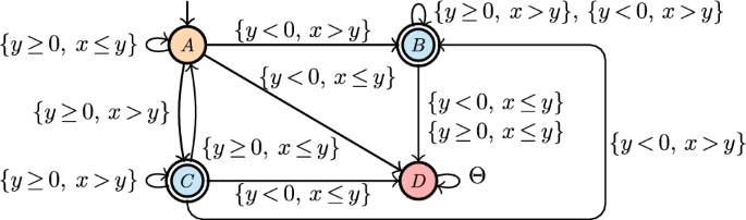
Anticipatory monitor for the formula (from [96]). is a shortcut representing all the constraints used in the automaton. Colors have the following meaning: orange means current violation, red permanent violation, and cyan current satisfaction (there is no state corresponding to permanent satisfaction for this formula)
An interesting future work building on the SMT-based anticipatory monitoring framework of [64] is to use it to extend the anticipatory monitoring approach for hybrid process specifications in [11]. There, a hybrid process specification consists of a collection of DPNs enriched with overarching constraints, but the approach deals with data using ad-hoc faithful data abstraction techniques, only defined for variable-to-constant conditions.
Another open problem is to consider richer datatypes, as done in [77] in the case of verification. We comment on this aspect in Sect. 7.1.
6.5.2 Predictive Monitoring
Predictive process monitoring [55] aims at predicting key indicators on the future of an ongoing process execution, such as likely outcome, expected completion time, which next activity will be selected, or even the entire continuation of the trace.
As surveyed in [55], a number of approaches, mainly based on neural networks, have been proposed to tackle this task, considering not only the sequence of activities in a trace, but also the data payload they carry. This makes predictive process monitoring compatible with the notion of data-aware trace given in Sect. 3.
A question that is instead still open relates to how models (in the context of this paper, data-aware process specifications) can be employed to improve predictions. A main direction is to use models as encoding background knowledge on the process, implicitly defining which traces are possible and which not. This is then instrumental to constrain predictions, ensuring that they are compatible with the provided background knowledge (e.g., that the predicted suffix conforms to the possible suffixes captured by the background knowledge). However, it is notoriously challenging to integrate hard/logical constraints in neural network architectures, a problem known under the term of neurosymbolic artificial intelligence [25, 92].
In the context of process mining, some initial attempts have been done in the direction where background knowledge is expressed using /Declare. One line of research focusses on teaching neural networks to perform classification [105, 106] or prediction [107] tasks compatibly with the given background constraints. Another line of research deals instead with explainability via counterfactual generations, aiming at producing counterfactual traces that are compatible with background constraints [29, 30]. Dealing with data-aware background knowledge, such as background constraints, is still an unexplored area.
7 Outlook
As summarised in this article, substantial progress has been made using SMT/OMT solving as a solid foundational and practical basis for tackling key data-aware process mining and analysis tasks: correctness checking and model repair, conformance checking, and (anticipatory) conformance monitoring. Notably, all the techniques overviewed here have been implemented in proof-of-concept prototypes:
- https://lindmt.unibz.it/ deals with correctness checking for general DPNs against full formulae, while https://ltl.adatool.dev and https://ctlstar.adatool.dev respectively tackle and its CTL extension that restrict the focus on DPNs with arithmetic datatypes.
- https://soundness.adatool.dev checks DPNs with arithmetic datatypes for soundness, providing repair facilities.
- https://monitoring.adatool.dev tackles anticipatory monitoring for the fragment of restricted to arithmetic datatypes.
- CoCoMoT for data-aware conformance checking of DPNs (including the extension with uncertainty) is available at https://github.com/bytekid/cocomot.
Such implementations have been subject to experimental tests mainly aiming at feasibility. A deeper investigation of their performance in real-life settings, as well as further insights on their application, constitute a natural continuation of this line of research, towards practical adoption.
Even from the foundational point of view, research in data-aware process mining is in its infancy. We then close by commenting on six timely lines where further research is required.
7.1 Dealing with Rich Datatypes
While verification of DPNs has been tackled for very general datatypes with mild model-theoretic assumptions [77], foundational and applied results for conformance checking, model repair, and monitoring, are currently limited to arithmetic datatypes. A natural extension is then to lift also these tasks to more general theories. These extensions are challenging and require genuinely novel research: while reasoning with arithmetic datatypes can rely on quantifier elimination techniques, this is not the case for more general theories [37]. A concrete direction to close this gap is to follow the route pursued in [77], in which quantifier elimination methods (previously exploited in [65,66,67] to deal with arithmetic datatypes) are now relaxed to uniform interpolation methods [37, 38].
7.2 Combined Discovery of Control-Flow and Data
As we have discussed in Sect. 6.1, contemporary techniques for data-aware process discovery first focus on the control-flow, and in a second step enrich it with data. Developing more tightly integrated techniques, able to discover at once the control-flow and data perspective, is an interesting avenue of unexplored research, which may potentially lead to discovery algorithms enjoying good properties such as re-discoverability, soundness, and perfect fitness.
7.3 Encodings and True Concurrency
All the presented techniques assume that concurrency is interpreted by interleaving. This opens up two open research questions. First, how to enrich the encodings with additional constraints reflecting the concurrency present in the process, which may be useful to implicitly break symmetries and, more in general, make the approaches faster in the case where the DPN under scrutiny has a high degree of concurrency. Second, how to deal with data-aware process mining by retaining true concurrency.
7.4 Handling Richer Datatypes in Process Mining
As discussed in the article, the advantage of adopting the SMT approach is that different theories can seamlessly be integrated. In principle, both DPNs and can indeed be subject to reasoning with richer datatypes than arithmetic, for example dealing with data structures. This is however an under-explored area of research in process mining as a whole, starting from the fact that (XES) event logs typically assume that even payloads are specified as simple key-value pairs. In addition, foundational research is missing on how to reassess key process mining tasks, such as conformance checking, in the light of richer datatypes.
7.5 Dealing with Object-Centric Logs
Object-centric process mining is rapidly becoming one of the main, novel areas of research in process mining [7, 24]. Some preliminary techniques have been devised to handle discovery [8] and conformance checking [84] for process models equipped with multiple objects related via one-to-many and many-to-many relations, but they are not yet able to deal with essential constructs such as multi-object synchronisation [24], as supported in formal representations for object-centric processes [12, 73, 98]. We foresee that the SMT/OMT approach can be extremely useful in pushing the boundaries of object-centric mining towards covering these essential constructs, again in the light of the fact that they natively support richer datatypes such as uninterpreted functions, arrays, and relations. Such richer datatypes are natively capable of handling multiple evolving objects and relations, and have already being exploited to capture object-centric [73] and relational data-aware processes [33, 36, 72]. A first step concretely witnessing this potential is [78], where conformance checking of object-centric processes is tackled using SMT/OMT, properly dealing with key modelling constructs that were out of reach before.
7.6 Neurosymbolic Techniques for Predictions
As pointed out in Sect. 6.5.2, techniques infusing background knowledge captured through data-aware process specifications inside predictive monitoring techniques is an interesting, completely open challenge. Neurosymbolic approaches are being increasingly researched in artificial intelligence to provide a solid foundational and algorithmic basis for this type of integration, but only few approaches are dealing with event and trace data. A key, technical question in this space concerns the logical representations of data-aware processes and their traces, as a common approach to support this integration is to move from a boolean/crisp setting to a fuzzy/probabilistic one. An initial step to realise this shift in a process mining setting is given in [56], where conformance checking of specifications on fuzzy event logs is studied – without covering at all the data perspective.