The BepiColombo mission (Benkhoff et al. 2010, 2021) is a significant effort to study Mercury and advance our understanding of the innermost planet in the solar system. Mercury, with a radius of , has a weak intrinsic magnetic field that can, to first order, be approximated as a dipole with a magnitude of about  and a northward offset of  (e.g., Alexeev et al. 2008; Anderson et al. 2012; Exner et al. 2024). The resulting magnetosphere is not only considerably smaller than Earth’s, but also highly dynamic due to the variability of the solar wind and the Interplanetary Magnetic Field (IMF) at Mercury’s orbital distance (Winslow et al. 2013). Many aspects of this Sun–planet interaction remain unresolved (Sun et al. 2022; Milillo et al. 2023).

BepiColombo will conduct a total of six flybys at Mercury before final orbit insertion, providing unique opportunities to study the planet’s magnetosphere. During these flybys, the spacecraft traverses magnetospheric regions and boundaries (Benkhoff et al. 2010; Mangano et al. 2021). The sixth Mercury flyby (often referred to as MSB6; Mercury Swing-By 6) will take place on January 8, 2025, and marks the final flyby before orbit insertion. The highly inclined trajectory will provide observations of Mercury’s high-latitude magnetosphere, crossing the nightside almost at the antisolar point, and is expected to pass through the tail plasma sheet. The unique geometry of this flyby, compared to earlier ones, makes it a particularly important target for investigation. Previous studies have examined earlier BepiColombo flybys, including Aizawa et al. (2023); Alberti et al. (2023); Fränz et al. (2024); Griton et al. (2023); Hadid et al. (2024); Harada et al. (2022, 2024); Robidel et al. (2023); Vecchio et al. (2024); Rojo et al. (2024); Exner et al. (2024); Teubenbacher et al. (2024).

The primary goal of this study is to establish a model-based reference for ion and magnetic field measurements during BepiColombo’s sixth flyby of Mercury and to understand how solar wind and IMF conditions influence ion dynamics. These references are crucial for interpreting the data collected by BepiColombo and for advancing the mission’s scientific objectives.

To achieve these goals, we employ a numerical hybrid plasma model, which is described in the following section. This model enables a kinetic description of ions, allowing the investigation of physical processes down to ion-kinetic length and time scales. Hybrid plasma modeling has been extensively applied to study Mercury’s magnetosphere, as demonstrated in numerous works, including Trávníček et al. (2007, 2009); Paral et al. (2010); Paral and Rankin (2013); Müller et al. (2011, 2012); Herčík et al. (2013); Fatemi et al. (2017, 2018, 2020, 2024); Exner et al. (2020, 2024); Jarvinen et al. (2020); Aizawa et al. (2021); Lu et al. (2022). In addition to studying the behavior of solar wind-origin protons in Mercury’s magnetosphere, we incorporate a sodium exosphere model (Exner et al. 2020) to model ion dynamics of exospheric particles. Assuming a neutral sodium gas profile and a constant ionization rate, sodium ions become subject to pick-up by the ambient electromagnetic fields [see Exner et al. (2020) for details]. A key strength of our model lies in its self-consistent treatment of exospheric particles, which dynamically influence the electromagnetic fields, unlike test-particle simulations that rely on static field models. This approach provides a more realistic representation of the coupled solar wind–magnetosphere–exosphere system.

The hybrid model AIKEF (Müller et al. 2012) (adaptive ion-kinetic electron-fluid) is used to model the global 3D interaction of Mercury with the solar wind. AIKEF has been used by various studies to model Mercury’s magnetosphere (Müller et al. 2012; Exner et al. 2018, 2020, 2024; Teubenbacher et al. 2024). We use three solar wind scenarios, based on the work from Dakeyo et al. (2022): a minimum, average, and maximum solar wind ram pressure to cover the expected solar wind variability (Winslow et al. 2013). Solar wind density, velocity, and temperature are changed in each case (see Table 1). The created bow shock waves are super-Alfvénic with Mach numbers  in all scenarios. We also include aberration by injecting the solar wind flow at an angle  depending on solar wind speed and the mean orbital velocity of Mercury; see Table 1. For the interplanetary magnetic field (IMF), we chose four probable Parker spiral scenarios (James et al. 2017), a planetward and a sunward direction, each pointing northward or southward, respectively. The IMF magnitude is set at , being the average value derived from MESSENGER (Solomon et al. 2007) data (James et al. 2017). We conduct a total of 12 simulations by combining the solar wind and IMF scenarios. The model time step is , where  is the gyration period of a solar wind proton. The spatial resolution is  and the simulation box size  ( is Mercury’s radius) in each direction. The planetary magnetic field is considered up to the octopole moment with coefficients  (Anderson et al. 2012; Exner et al. 2024).

All simulations are initialized with a sodium exosphere model implemented by Exner et al. (2020), adopting model parameters from Gamborino et al. (2019). It assumes a constant sodium neutral density profile resulting from the major processes that generate the exosphere (Gamborino et al. 2019). A constant ionization frequency simulating photoionization then ionizes neutral particles; see Exner et al. (2020) for more details. The resulting sodium ions are accelerated by the Lorentz force and propagated self-consistently in the simulation.

After quasi-stationarity is reached (after about 3–5 solar wind simulation box passes) in all 12 scenarios, we extract the modeled ion data along the MSB6 trajectory. We compute the omnidirectional differential ion energy flux, Teubenbacher et al. (2025) over a range from 10 eV to 40 keV in 50 logarithmic energy bins for protons and sodium ions, respectively. The fluxes are computed along the MSB6 trajectory at 100 km spacings. Additionally, we extract magnetic field and proton velocity data from the model runs to facilitate the interpretation of the simulated ion spectra.

The model employs the Mercury Anti-Solar Orbital (MASO) coordinate system, including aberration effects. In this system, the z-axis is defined as the positive normal to Mercury’s orbital plane and is anti-parallel to the planet’s magnetic dipole moment. The y-axis points in the direction of Mercury’s orbital motion (i.e., toward dawn), while the x-axis is approximately aligned with the solar wind velocity, directed anti-sunward with an angular offset due to aberration. This coordinate system can be converted into the commonly used Mercury Solar Orbital (MSO) system by inverting the signs of the x- and y-components.

Our hybrid simulations of Mercury’s magnetosphere provide modeled ion and magnetic field data as a reference for comparison to measurement data obtained during BepiColombo’s sixth Mercury flyby. In Fig. 1, we show our results for the minimum (top three panels), average (middle three panels), and maximum solar wind cases (bottom three panels). For each case, we plot the omnidirectional differential ion energy flux of protons (H) and sodium ions (Na). To facilitate comparison, the fluxes of the different ion populations are displayed in separate plots, with the other species shown as a gray background for context. For example, we present the ion data for the planetary-southward IMF case. In addition, magnetic field data are displayed for each solar wind scenario. For the planetary-southward IMF case, the magnetic field is represented by solid lines. At the same time, the shaded areas indicate the minimum and maximum values across all IMF cases, highlighting the variability resulting from changes in IMF input. While the ion energy spectra also vary across different IMF configurations, the planetary-southward IMF case is shown here as a representative example, and spectra for all scenarios are included in the supplementary material for reference. The vertical lines and shaded areas denote the bow shock (BS), magnetopause (MP) and tail current sheet (CS) crossings, again across all IMF cases. Detailed timings for all 12 simulation runs are summarized in Table 3.

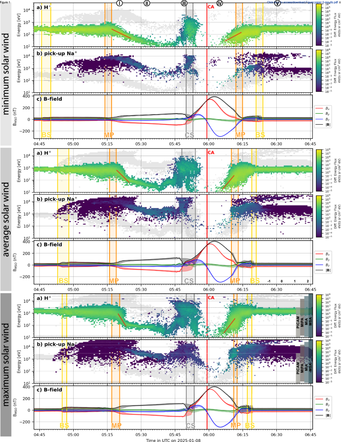
Simulation results for BepiColombo’s sixth Mercury flyby for the planetward-southward IMF case: the top three panels show the results for minimum solar wind input, the middle three panels for average solar wind input, and the bottom three panels for maximum solar wind input. Energy ranges of relevant ion instruments onboard BepiColombo are marked with PICAM, MIPA, MIA and MSA and described in the text. Ion data are presented for a protons and b sodium ions. For the planetary-southward IMF case, the magnetic field (c) is depicted with solid lines, while shaded areas indicate the minimum and maximum values across all IMF scenarios. Boundary crossings and the closest approach (CA) are marked with vertical lines, and regions I–V are highlighted as described in the text

Full size image

To aid interpretation, Fig. 1 shows the energy ranges of the ion instruments onboard BepiColombo relevant to this study: the Planetary Ion Camera (PICAM) and the Miniature Ion Precipitation Analyzer (MIPA) onboard the SERENA suit (Orsini et al. 2021) onboard the MPO spacecraft and the Mass Spectrum Analyzer (MSA) and Mercury Ion spectral Analyzer (MIA) as part of the Mercury Plasma Particle Experiment [MPPE, Saito et al. (2021)] onboard the MMO/Mio spacecraft.

To set the energy spectra in a spatial reference, Fig. 2 illustrates the meridional plane of the  and  (MASO) proton velocity components for each of the solar wind scenarios, specifically for the planetary-southward IMF case. BepiColombo’s MSB6 trajectory is overplotted in each panel of the figure. A key point to consider is that this plot represents a projection of the trajectory onto the meridional plane, which provides a suitable approximation for the MSB6 flyby geometry (see inset in Fig. 2b).

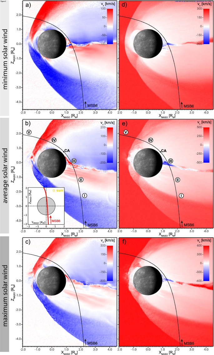
Simulation results for BepiColombo’s sixth Mercury flyby under planetary-southward IMF conditions. Panels are grouped by solar wind input: minimum (a, d), average (b, e), and maximum (c, f). All plots show the MSB6 trajectory and the  (a–c) and  (d–f) proton velocity components projected on the meridional xz-plane; regions I–V are labeled as described in the text and CA is the closest approach. The inset in b shows the MSB6 trajectory in the YZ-plane for reference

Full size image

Based on the simulation results, the spacecraft’s high-latitude trajectory during MSB6 led to similar magnetospheric region crossings across all modeled upstream solar wind and IMF conditions. Nevertheless, the energies and spatial locations of the different particle populations vary between scenarios. For instance, the inbound bow shock crossing time differs by up to 12 min, with the earliest crossing at 04:46 UTC in the minimum solar wind and planetary-southward (PS) IMF case, and the latest at 04:58 UTC in the maximum solar wind and sunward-southward IMF case. Consistent with previous analyses of spacecraft observations (Winslow et al. 2013) and earlier numerical modeling studies (e.g., Exner et al. 2018; Lai et al. 2024), the simulation results show that the bow shock becomes increasingly confined with higher solar wind Mach numbers. This behavior is reflected qualitatively in the decreasing temporal separation between the inbound and outbound bow shock crossings: a smaller time interval indicates a more compressed bow shock structure. A similar dependence is seen for the magnetopause, whose position varies with the solar wind ram pressure (Winslow et al. 2013; He et al. 2017), as illustrated in Fig. 1.

Focusing on the average solar wind case in Figs. 1b and 2b, regions (I–V) are defined and will be discussed in the following paragraphs. Starting with the spacecraft approaching from the south, it enters the magnetosheath through the bow shock. The local plasma population is decelerated and thermalized, resulting in a broader energy distribution indicative of a wider flux spread and elevated temperatures (05:00–05:15 UTC).

4.1 Region (I): southern plasma mantle (solar wind-dependent thickness and slope)

After crossing the magnetopause almost perpendicularly, the southern tail lobe region is entered. Just beyond the magnetopause, an energy dispersion-like feature appears, marked as region (I), where proton energies decrease by about one order of magnitude. This feature is identified as the plasma mantle, representing the transition region from magnetosheath plasma to lobe plasma (DiBraccio et al. 2015; Jasinski et al. 2017). At high latitudes, particles travel tailward along magnetic field lines, with higher-energy ions moving faster parallel to the field, while the  drift preferentially affects lower-energy ions. Consequently, higher-energy ions remain closer to the magnetopause, whereas lower-energy ions are observed farther tailward, creating a characteristic energy dispersion slope (Jasinski et al. 2017). These slopes are marked with red lines in the proton flux panels of Fig. 1. The simulations show that the slopes steepen and the thickness of the boundary layers increases as the magnetosheath particle energy increases. Since the IMF direction and strength remain fixed in the particle energy spectra in Fig. 1, the steepening is directly attributed to higher solar wind input energy. This is schematically illustrated in Fig. 3a for the minimum and Fig. 3b for the maximum solar wind case.

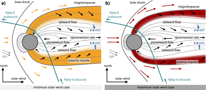
Schematic of the convection patterns during planetary-southward IMF in the meridional plane. a (left) shows minimum solar wind conditions and b (right) maximum solar wind conditions

Full size image

From the spacecraft velocity at the time of the boundary crossing (approximately 2.6 km/s) and the time interval of the dispersion signature, assuming a perpendicular crossing, the estimated plasma mantle thicknesses  are listed in Table 2. Compared to Earth, these values place Mercury’s modeled mantle near the lower end of the observed range when scaled by planetary radius. At Earth, plasma mantle thicknesses typically range from 0.5 to 4  (Rosenbauer et al. 1975). It is important to note, however, that mantle thickness increases with downtail distance (Rosenbauer et al. 1975; Jasinski et al. 2017). The MSB6 trajectory intersects the mantle relatively close to the planet at , where the mantle appears broader under weaker solar wind conditions (see Table 2). This suggests that the expansion fan (i.e., the plasma mantle) flares more rapidly downtail when the solar wind input is reduced.

The drift velocity  and magnetic field strength around the mantle crossing  remain nearly constant across all solar wind cases due to the fixed IMF magnitude of 25 nT. However, the parallel velocity  of magnetosheath protons is lower under minimum solar wind conditions, leading to broader mantle regions and more diffuse boundaries with the convection lobe (see region I in Fig. 1). In contrast, stronger solar wind conditions yield higher  values, resulting in faster downtail escape, narrower mantle regions, and sharper transitions, clearly visible as steeper slopes in the energy–time dispersions in Fig. 1. The average cross-tail electric field as described by DiBraccio et al. (2015) is estimated as , yielding . The corresponding cross-magnetospheric electric potentials are computed via , where  is the tail width. These widths are consistent with the average value of  reported by Winslow et al. (2013), and the resulting potentials lie within the expected range of  for , as estimated by Jasinski et al. (2017). Furthermore, the cross-tail electric fields and cross-magnetospheric electric potentials estimated by DiBraccio et al. (2015) are consistent with the range of values obtained in our simulation.

4.2 Region (II): southern lobe ( drift convection)

Region (II) marks the southern lobe, where energy and particle flux decrease slightly as the spacecraft approaches the equator. Protons here exhibit energies between 20–200 eV, while sodium ions coming from the southern cusp region convect mostly tailward with energies between 300–5000 eV. The observed energy difference approximately scales with the mass ratio of the two species.

Investigating the proton flow directions in Fig. 2, several features are apparent. In the southern lobe region, the electric field points northward and duskward, while the magnetic field is directed predominantly planetward (the field vectors are omitted here to improve visual clarity). This configuration results in an  drift that causes ions to flow northward and dawnward. In the northern lobe, the electric field points largely in the same direction; however, the magnetic field is oriented tailward. Consequently, the resulting  drift of the protons is directed southward and duskward. Along the MSB6 trajectory in the southern lobe, the  drift velocity decreases with increasing proximity to the planet, due to the strengthening of the planetary magnetic field. A dispersion signature can also be observed in this region, similar to that in the plasma mantle but exhibiting a much shallower slope (see Fig. 1, Region II). The ion flow patterns can be seen in Fig. 2a–c, and are schematically illustrated in Fig. 3a and b for the minimum and maximum solar wind cases, respectively.

4.3 Region (III): tail current sheet (fast planetward plasma flow)

Region (III) corresponds to the mean passage through the tail current sheet. Multiple proton populations are observed: a main population centered around 1 keV, and two lower energy populations near 05:44 UTC and 05:50 UTC at approximately 100 eV. This behavior is interpreted as a crossing of the plasma sheet, where it separates into the plasma horns (Glass et al. 2022), marked by a sign reversal of the  component at around 05:49 UTC, followed by a “grazing” of the northern plasma horn near 05:53 UTC. In the hybrid model, current sheets can become thicker than in reality due to the spatial limit around ion kinetic scales. Therefore, a “grazing” of current sheet structures is possible. The lower energy populations around 100 eV likely represent signatures of lobe plasma. Notably, these features become more distinct with increasing solar wind intensity: while proton populations around the current sheet are clearly resolved in the maximum solar wind case (Fig. 1, bottom panel a), they are barely visible in the minimum solar wind scenario (top panel a). The energies of sodium ions in the current sheet increase accordingly, ranging from 0.5–10 keV (minimum solar wind), to 1–20 keV (average solar wind), and 1–30 keV (maximum solar wind).

The current sheet/plasma horn passage can also be seen in Fig. 2a–c, marked with (III). The northern plasma horn seems more pronounced than the southern one in the average simulation scenario in b. A similar signature can be seen in c for the maximum solar wind case. In contrast, in a, a clear splitting of the tail current sheet into northern and southern horns can be seen, with strong positive and negative  components. It is important to note that the panels of Fig. 2 only show a momentary picture of one velocity component in one plane, respectively.

Due to the drifts toward the central current sheet (see Fig. 2a–c), in addition to an overall downtail field-aligned velocity, from both tail lobes, the central plasma sheet is fed with particles that are accelerated tailward and planetward. This acceleration is consistent with magnetic reconnection occurring in the near-tail region, as resolved in the simulation. Figure 2d–f illustrates the corresponding reconnection geometry, where planetward-flowing ions are shown in blue and tailward-moving ions in red. The modeled X-line in the meridional plane is located at around  in the minimum solar wind case (d) and at about  in the maximum solar wind case (f). In the average solar wind case, the X-line is located at . However, this is likely just a snapshot of tail dynamics evolving in the simulation, i.e., a plasmoid might separate and move in a tailward direction starting at about , creating a new X-line there. The particle velocities of particles accelerated planetward in the tail current region even exceed solar wind speeds, which is evident in the energy spectra in Fig. 1.

4.4 Region around CA: northern lobe, near-planet (low plasma density)

Following the current sheet crossing, the spacecraft enters the northern lobe. Near closest approach (05:54–06:05 UTC), denoted with (CA), proton and sodium ion densities are low, and the flux is minimal compared to the southern lobe. This is consistent with the near-zero proton background reported in MESSENGER observations of the northern lobe (Glass et al. 2022) and the lobe region more generally (Jasinski et al. 2017). For the low-density proton population present in this region, the  drift (as explained above) is directed southward and duskward. These flow patterns are visible in Fig. 2a–c, and are schematically illustrated in Fig. 3. It should be noted that close to the planet, additional drifts—such as curvature and gradient drifts—as well as other acceleration processes, also contribute to the overall particle motion.

4.5 Region (IV): northern magnetopause structure (cusp dispersion-like signature)

After 06:05 UTC, region (IV), a proton energy dispersion-like signature from 20–1000 eV is observed, again interpreted as the plasma mantle in high-latitude regions close to the planet. The populations seen here also resemble the northern cusp region, where the plasma originates from the magnetosheath and particles either flow away from the planet downtail or they precipitate onto the surface; see Fig. 2a–c at . Immediately afterward, the magnetopause is crossed outbound into the magnetosheath. In the maximum solar wind case, a distinct sodium ion population appears between 06:09 and 06:12 UTC, with energies of 1–10 keV, indicative of ions escaping along open field lines. Following a brief passage through the magnetosheath, the spacecraft exits the magnetosphere via the bow shock and re-enters the solar wind.

4.6 Region (V): upstream solar wind (pick-up sodium ions)

Region (V) shows the solar wind input in the proton energy spectra in Fig. 1, resembling the input velocities from Table 1. Additionally, two faint signatures of sodium ions that are ionized upstream of the bow shock and subsequently picked up by the solar wind can be seen. Under average solar wind conditions (middle panel in Fig. 1), the lower-energy population appears at around 3 keV (corresponding to approximately 160 km/s) and represents newly picked-up sodium ions. In contrast, a second, higher-energy population shows Na energies in the range of 10–20 keV (corresponding to 290–410 km/s). These higher-energy ions likely originate from reflection at the bow shock and are accelerated along the mostly northward-pointing convective electric field, , where  is the solar wind velocity and  the interplanetary magnetic field vector, as given in Table 1. Sodium ions subsequently reach the high-latitude region of the MSB6 spacecraft trajectory due to their large gyroradii on the order of 2800–3900 km. In contrast, high-energy protons are not observed along the MSB6 spacecraft trajectory in the solar wind, possibly due to the significantly smaller proton gyroradii.

When comparing the energy of the modeled particle populations to the energy ranges of the onboard particle instruments, two key observations emerge: (1) the sodium ion energy flux is consistently lower than that of the protons, and (2) cross-comparison between different instruments will be essential, given the limitations of their respective energy ranges. We also want to emphasize again that actual measurements may deviate from the modeled results, not only due to systematic and stochastic uncertainties, but also owing to instrumental field-of-view constraints.

Finally, Table 3 summarizes the modeled timing of key magnetospheric boundary crossings during BepiColombo’s sixth Mercury flyby on January 8, 2025. The inbound bow shock is predicted to occur between 04:46 and 04:58 UTC, followed by the inbound magnetopause crossing between 05:14 and 05:20 UTC. The outbound magnetopause is crossed between 06:10 and 06:15 UTC, with the outbound bow shock occurring between 06:17 and 06:24 UTC. The tail current sheet crossing is centered between 05:48 and 05:54 UTC and lasts approximately 10 min, as indicated by the extent of population (III) in Fig. 1.