Polarization is a fundamental property of electromagnetic (EM) waves, representing the orientation of the electric field oscillations perpendicular to the wave propagation direction. Effective manipulation of polarization plays a critical role in various applications, including antenna design (Duan et al. 2016; Zhang et al. 2019), biomedical sensing (Maurya and Singhal 2024), and radar technologies (Dutta et al. 2021; Jia et al. 2015). Consequently, controlling the polarization state of EM waves has attracted significant research interest.

Traditional approaches for polarization control have employed mechanisms such as the Faraday effect (Meissner and Wentz 2006), total internal reflection (Petrov 2007), and optical gratings (Gimeno et al. 1994). However, these methods often suffer from limitations including narrow bandwidths, bulky structures, and considerable losses. Therefore, novel solutions offering compact size, ease of fabrication, and enhanced polarization performance are still highly sought after.

Recently, metasurfaces, which are planar (two–dimensional) forms of metamaterials, have emerged as promising candidates for polarization conversion. Compared to conventional polarization converters, metasurfaces offer advantages such as reduced fabrication complexity, lower cost, and simpler structural design. They enable control over the phase, amplitude, and polarization of EM waves across a wide frequency range spanning microwave (Zeng et al. 2019; Turkmen-Kucuksari 2023a), terahertz (Das and Mandal 2022; Tao et al. 2023; Barkabian et al. 2021; Cheng and Li 2022), and infrared (Johnson et al. 2006) spectra.

Existing literature reveals that polarization converters based on metasurfaces can operate either in transmission (Ghosh et al. 2021; Ako et al. 2020) or reflection modes (Zheng et al. 2015; Turkmen-Kucuksari 2023b; Yang et al. 2018; Bilal et al. 2020). Several converter types have been reported, including linear–to–linear (LTL) (Nagini and Chandu 2023), linear–to–circular (LTC) (Shukoor et al. 2022), linear–to–linear/circular (Turkmen-Kucuksari 2023a, 2023b), and circular–to–linear (CTL) (Shao et al. 2018) converters. These designs may be realized as single–layer (Tao et al. 2023; Zang et al. 2018; Pan et al. 2023) or multilayer structures (Zeng et al. 2019).

Polarization converters operating in the terahertz (THz) band have been less extensively explored compared to their microwave counterparts. Among them, reflective polarization converters provide a simpler design alternative to transmissive types (Cheng et al. 2016). Motivated by this, the present study investigates a multifunctional reflective multiband polarization converter designed for the THz range, with potential applications in communications, spectroscopy, and biomedical fields (Nagini et al. 2024; Phan et al. 2024; Wang et al. 2024).

In prior works, an axial ratio (AR) of ≤ 3 dB is frequently employed to define the LTC conversion bandwidth, while a polarization conversion ratio (PCR) of ≥ 0.9 is typically used to identify LTL conversion bands (Zeng et al. 2019; Cheng et al. 2016). Our analysis indicates that the determination of LTC conversion regions should not rely solely on the axial ratio (AR), but also consider other criteria such as the phase difference parameter (∆φ_xy). Similarly, for accurately identifying LTL conversion bands, both the polarization conversion ratio (PCR) and phase difference (∆φ_xy) criteria must be evaluated simultaneously.

In applications demanding exceptionally low polarization distortion, such as satellite communications, advanced radar systems, and high–data–rate wireless links, a stricter AR threshold of 1 dB is preferred (Wen et al. 2020). Therefore, this study adopts AR ≤ 1 dB along with ∆φ_xy ± 5° as criteria for LTC regions, which are identified at 0.449–0.455 THz, 0.5404–0.8049 THz, and 1.182–1.587 THz. For LTL regions, PCR ≥ 0.9 combined with ∆φ_xy ± 5° defines the operational narrow bands at 0.4906–0.4912 THz, 0.9739–0.9743 THz, and 1.699–1.702 THz. Although these LTL bands are narrow, they are suitable for frequency–selective THz sensing and notch filtering applications, where high spectral resolution is essential (Redo-Sanchez and Zhang 2008).

Finally, due to the limited availability of fabrication facilities in the THz range, this work relies on well-established analytical and numerical modeling methods commonly accepted in the literature (Bilal et al. 2020; Nagini and Chandu 2023; Shukoor et al. 2022; Jiang et al. 2017; Majeed et al. 2024) to realize and validate the design.

The unit cells of three different metamaterial polarization converter structures are shown in Fig. 1, which are formed by placing metal patterns with splits of different sizes with a metal thickness of 0.4 μm on a polyimide substrate. The conductivity of the gold is equal to 4.561 × 10⁷ S/m. The thickness, dielectric constant, and loss tangent of the polyimide substrate are equal to 26 μm, 3.5 and 0.0027, respectively. In the figures, the yellow–colored parts are gold, and the gray–colored parts are the dielectric plates. The polarization converter, Design–I, has one ring with two diagonal slits as in Fig. 1a. The polarization converter Design–II is obtained by placing another ring with two diagonal slits inside the Design–I polarization converter, as shown in Fig. 1b. Polarization converter III (i.e., the final design) is obtained by inserting an additional patch with a diagonal slit inside the Design–II polarization converter as shown in Fig. 1c.

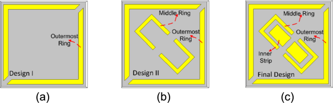
a Design–I with one ring, b design–II with two rings, c final design

Full size image

The design parameters are shown in Fig. 2a on the unit cell of the final design with three rings. The thicknesses of the outermost (w₁) and middle (w₂) rings are 4 μm and 3 μm, respectively. The separations named s₁ and s₂ are equal to 4 μm and 2 μm, respectively. The gap of the outermost ring (g₁), middle ring (g₂), and inner patch (g₃) are 4 μm, 7 μm, and 4 μm, respectively. Side lengths of the metal parts are r₁ = 66 μm, r₂ = 50 μm, r₃ = 20 μm, r₄ = 10 μm and r₅ = 36 μm. p = 70 μm is the lengths of the unit cell in the x and y directions.

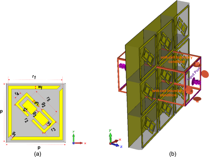
a Design parameters, b simulation setup

Full size image

CST Microwave Studio software is utilized for simulations of the structure. During the simulations, the polarization converter unit cell is placed in the center of the computational volume with dimensions p in x– and y–directions. The designed structures are excited by planar electromagnetic waves. In the setup shown in Fig. 2b, the y–axis–oriented electric field (E), x–axis–oriented magnetic field (H) and z–axis–oriented propagation (k) vectors were determined. The outer surfaces of the computational volume perpendicular to the propagation vector (k) are defined as input and output ports, while the other outer surfaces are bounded by periodic (i.e. unit–cell) boundary conditions. These periodic boundary conditions allow the simulation of a two–dimensional periodic structure consisting of an infinite unit cell in the plane containing the electric and magnetic field components of the electromagnetic wave. The distance in the z–direction was automatically determined for the simulation by the CST Microwave Studio software, which was optimized with respect to the upper frequencies. For the lower and upper frequencies of the simulation setup, frequencies 0.2 THz and 2.5 THz were used, respectively.

Polarization converters made using metamaterials can have two different modes based on reflection or transmission. The proposed polarization converter, having a fully metallic backing, operates as a reflective polarization converter. Thus, the analysis of reflected waves enables the determination of polarization states. Reflected electric fields can be related to incident waves by the notation in Eq. (1).

 is defined as the x–polarized reflected electric field.  field is defined as the y–polarized reflected electric field. The incident electric fields are  and  for x and y polarizations, respectively. For the x–polarized incoming wave, r_xx refers to the co–polarized components, while r_yx refers to the cross–polarized components. For the y–polarized incoming wave, r_yy (see Eq. 2) denotes the co–polarized components, while r_xy (see Eq. 3) denotes the cross–polarized components. It is essential to note the design’s diagonal symmetric geometry, which results in similar behaviors for x–polarized and y–polarized incident waves. Therefore, in the rest of the section, equations will be provided solely for y–polarized incident waves.

One of the parameters used to decide the polarization conversion state is the amplitude ratio, given in Eq. 4. In an ideal LTL and LTC transformation, it is desirable for the amplitude ratio to be equal to zero and one, respectively.

Another parameter evaluated to decide the polarization conversion state is Δφ_xy, as given in Eq. 5. For a perfect LTL conversion, the phase difference ∆φ_xy equals nπ, where n is an integer. On the other hand, for a perfect LTC transformation, ∆φ_xy equals nπ/2, where n is an odd integer. In addition, reflection coefficient magnitudes around 0.7 indicate an LTC polarization conversion behavior.

The PCR, as given in Eq. 6, is another parameter often used to decide the polarization conversion state. For an ideal LTL and LTC conversion, the PCR should be 1 and 0.5, respectively (Turkmen-Kucuksari 2023a, 2023b).

The ellipticity ratio e given in Eq. 7, which is one of the parameters used to decide the polarization conversion state, should ideally be 0 and ± 1 for LTL and LTC conversions, respectively. Ellipticity angle () is also given in Eq. 8 (Wei et al. 2023). In this work, the  is defined following the IEEE convention, where right–handed circular polarization (RHCP) corresponds to + 45° and left–handed circular polarization (LHCP) corresponds to − 45°. A γ value of 0° indicates ideal LTL polarization.

The axial ratio (AR) given in Eq. 9 is also often used to evaluate the polarization conversion state and should be ∞ for LTL conversion and 1 (i.e., 0 dB) for LTC conversion.

In Eq. (9), a is

The reflection coefficients and phase values for Design I, Design II and Final Design are represented in Fig. 3a and b, respectively. As seen in Fig. 3a and b, the reflection coefficients and phase values of three designs are almost the same over the bandwidth of 0.2 THz–1.41 THz. The additional middle ring mainly modifies the behavior of the Design I beyond 1.41 THz. Besides, an additional inner strip used in Final Design modifies the behavior of the Design II beyond 1.71 THz. As seen in Fig. 3a, reflection coefficient values around 0.7 imply LTC polarization conversion, which occur at frequencies around 0.45, 0.67 THz, 1.4 THz, 1.8 THz and 2.13 THz for the Final design. As seen in Fig. 3a, around 0.48 THz, 0.97 THz and 1.7 THz, the co–polarized reflection coefficient ≈ 0 and the cross–polarized reflection coefficient ≈ 1 simultaneously for final design. In this case, LTL polarization conversion occurs. The amplitude ratio, phase differences, PCR, AR, and ellipticity parameters should be evaluated simultaneously to clarify the LTL and LTC conversion bands (Turkmen-Kucuksari 2023a, 2023b).

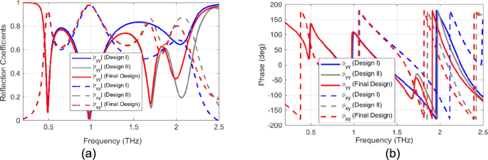
a Reflection coefficients. b Phase values of the reflections

Full size image

Figure 4a shows the AR of the designs. The phase difference (Δφ_xy) values are given in Fig. 4b. AR ≤ 1 dB is satisfied over the five bands: (0.448–0.459 THz), (0.5404–0.8049THz), (1.182–1.587 THz), (1.794–1.9 THz) and (2.109–2.162 THz) for Final Design. The first and second bands are almost similar in all designs. Bands (1.17–1.31 THz) and (1.85 – 2.14 THz) are also LTC conversion bands for Design I, considering AR ≤ 1 dB criteria. The LTC conversion band over (1.182–1.587 THz) is preserved for Design I and Design II. For Design II, (1.808–1.916 THz) and (2.203–2.245 THz) are the fourth and fifth LTC conversion bands. At the resonance frequencies where LTL polarization conversion occurs (i.e., 0.48 THz, 0.97 THz, and 1.7 THz), the axial ratio (AR) exceeds 16 dB.

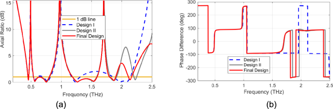
a Axial ratio of the proposed design in dB, b Phase differences

Full size image

The simultaneous satisfaction of AR ≤ 1 dB and ∆φ_xy = nπ/2 ± 5° (n = 1, ± 3, ± 5…) is used as a design criterion for a nearly ideal LTC polarization conversion. Considering simultaneously AR ≤ 1 dB and ∆φ_xy = nπ/2 ± 5° (n = 1, ± 3, ± 5…), the bands for an ideal LTC conversion are (0.449–0.455 THz), (0.5404–0.8049 THz), (1.182 – 1.587 THz), (1.861 –1.9 THz) for Final Design. Also, over the bandwidth of (2.109–2.162 THz), the case ∆φ_xy = nπ/2 ± 7° occurs for Final Design. Furthermore, for Design II, ∆φ_xy = nπ/2 ± 10° (n = 1, ± 3, ± 5…) is satisfied over (1.808–1.916 THz) and (2.203–2.245 THz). The reflection phase shown in Fig. 4b decreases with increasing frequency, which is a typical behavior for resonant or dispersive metasurface structures. This frequency–dependent phase response is particularly important for applications such as beam steering, phase compensation, and dispersion engineering (Pfeiffer and Grbic 2013).

The PCR values for three designs are presented in Fig. 5a. Within the bandwidths of LTC conversion, PCR values around 0.5 are observed, corresponding to the bands assigned by the evaluation of AR values. For the final design, a polarization conversion ratio (PCR) of 0.5 ± 0.11 is achieved across the LTC polarization conversion bands of 0.449–0.455 THz, 0.5404–0.8049 THz, and 1.182–1.587 THz. Additionally, PCR ≥ 0.9 is widely employed to define bands of LTL polarization conversion (Yang et al. 2018; Nagini and Chandu 2023; Shukoor et al. 2022). PCR values higher than 0.9 are found within the bands of (0.478–0.505 THz) and (0.917–1.052 THz) for all designs. Design II has two additional LTL conversion bands, namely (1.666–1.742 THz) and (2.006–2. 123 THz). Final Design has an additional LTL conversion band such as (1.666–1.723 THz). As seen in Fig. 4a, AR ≥ 4.81 dB is satisfied within the LTL conversion bands assigned by the evaluation of PCR values. The LTL conversion bands (0.478–0.505 THz), (0.917–1.052 THz) and (1.666–1.723) for Final Design, which are considered as LTL conversion bands by evaluating the PCR values, have a maximum deviation of 75°, 88° and 49°, respectively, from the condition ∆φ_xy = nπ (n = 0, ± 1, ± 2…). It is clear that the phase difference values in this range are far from the ∆φ_xy = nπ (n = 0, ± 1, ± 2…) criterion. If we choose the design criterion as ∆φ_xy = nπ ± 5° (n = 1, ± 2, ± 3…), there are three very narrow LTL conversion bands over (0.4906–0.4912 THz), (0.9739 –0.9743 THz) and (1.699–1.702 THz). Thus, ∆φ_xy and PCR must be considered simultaneously to correctly identify the LTL region.

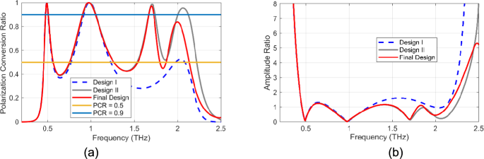
a Polarization conversion ratio, b Amplitude ratio

Full size image

Figure 5b shows the amplitude ratio of the designs. Amplitude ratio values close to one, as expected, indicating LTC conversion, are obtained around frequencies 0.45 THz, 0.67 THz, 1.4 THz, 1.8 THz, and 2.13 THz. Amplitude ratio values close to zero, indicating LTL conversion, are also obtained around frequencies 0.48 THz, 0.97 THz, 1.7 THz, and 2.1 THz. It should be noted that a more stable amplitude ratio distribution after 1.31 THz is achieved in the Final Design and Design II compared to Design I. As seen in Fig. 3a, the reflection coefficients (|r_yy| and |r_xy|) undergo considerable changes among Design I, Design II, and the Final Design. However, the amplitude ratio which is used in determination of the AR, remains similar in multiple frequency regions across all three designs, as shown in Fig. 5b. This is because both co– and cross–polarized components scale proportionally in many bands, especially where resonance strength or symmetry is preserved. Notable differences appear mainly above 2.1 THz, where additional structure in the Final Design alters the coupling.

e being + 1 and –1 indicates right–hand circular polarization (RHCP) and left–hand circular polarization (LHCP), respectively. e ≈ ± 1 with a maximum deviation of 0.03 is found within the four LTC conversion bands of (0.449–0.455 THz), (0.5404–0.8049THz), (1.182–1.587 THz), (1.861–1.9 THz) for Final Design as seen in Fig. 6. Among these bands, LHCP behavior (e ≈ –1) is observed in (0.449–0.455 THz) and (1.182–1.587 THz), while RHCP behavior (e ≈ + 1) is observed in (0.5404–0.8049 THz) and (1.861–1.9 THz). Besides, e ≈ 0 with a maximum deviation of 0.02 is found within the three LTL conversion bands of (0.4906–0.4912 THz), (0.9739–0.9743 THz) and (1.699–1.702 THz). Figure 6 shows that γ attains ± 45° (± 5° deviation) across the four LTC conversion bands, whereas in the three LTL bands, γ is centered around 0° with a maximum deviation of 1.5°.

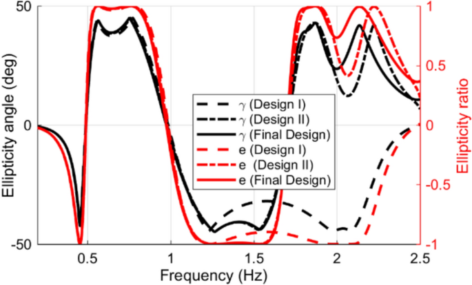
Ellipticity ratio (e) and ellipticity angle () of the proposed design

Full size image

To gain deeper insight into the polarization conversion behaviour, the incident and reflected electromagnetic fields are resolved into two orthogonal basis vectors, namely the u and v components. The u–v coordinate framework is defined by rotating the conventional x–y axes by 45 degrees around the z–axis, as depicted in Fig. 7. As depicted in Fig. 7, an incident electromagnetic wave with y–axis polarization can be resolved into two orthogonal components, denoted as  and , aligned along the u–axis and v–axis, respectively. This decomposition facilitates the analysis of the polarization conversion process, and the incident wave can be mathematically represented as follows (Majeed et al. 2024):

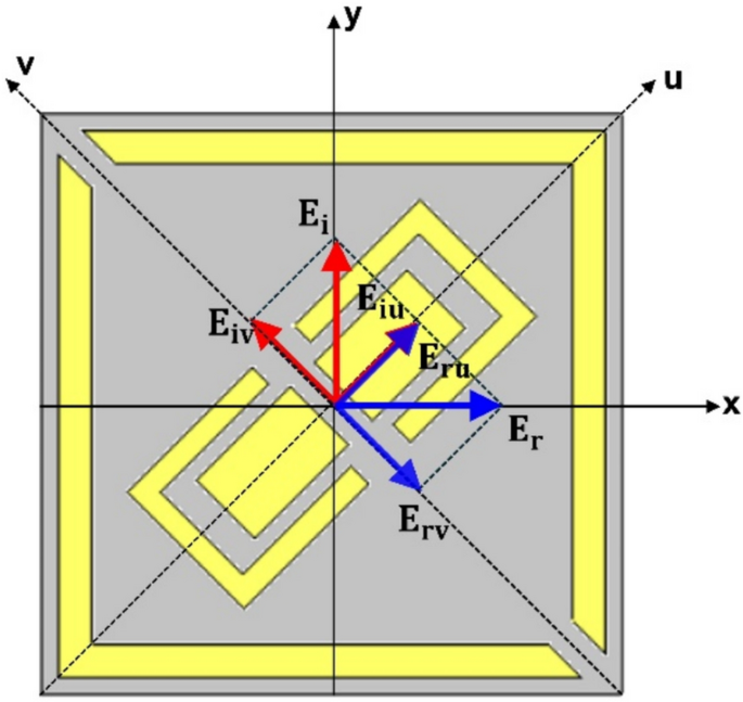
Schematic view of the polarization conversion process

Full size image

Upon reflection by the polarization converter, the incident electromagnetic wave undergoes a transformation, resulting in a reflected wave that can be characterized by the following expression (Majeed et al. 2024):

In this context, the reflection coefficients , ,  and  represent the amplitudes corresponding to the polarization conversions from u–to–u, u–to–v, v–to–u, and v–to–v, respectively. The associated reflection phases are denoted as , ,  and . When the cross–polarization reflection coefficients satisfy  and the co–polarization reflection coefficients are equal, i.e., , with a phase difference  where n is an integer, the reflected electric field  can be expressed as:

Under these conditions, the reflected wave exhibits circular polarization characteristics. The asymmetric design of the proposed polarization converter introduces anisotropic electromagnetic properties. This anisotropy leads to distinct reflection behaviours along the orthogonal u– and v–axes, resulting in variations in both the magnitude and phase of the reflected electromagnetic waves in these directions. As illustrated in Fig. 8, the phase difference  is close to ± 90° over the three bands: (0.449–0.455 THz), (0.5404–0.8049 THz), and (1.182–1.587 THz) which indicating the achievement of linear–to–circular (LTC) polarization conversion for the final design. The axial ratio for u–v and x–y polarized waves exhibits similar behavior, as shown in Fig. 8c.

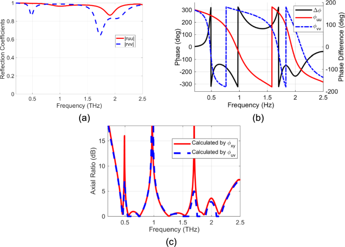
a Reflected amplitudes corresponding to co and cross–polarization components. b Phase of co–polarized electric field components (left). Phase difference between co–polarized electric field components along the u– and v–directions (right). c Axial ratio in dB

Full size image

To investigate the underlying polarization conversion mechanisms for both LTL and LTC, surface current distributions on the top metallic structure and the ground plane were analysed in the u–v coordinate system at three representative resonance frequencies: 0.49 THz (for LTL), 0.80 THz (for RHCP), and 1.185 THz (for LHCP), as shown in Fig. 9 (Jiang et al. 2017; Majeed et al. 2024). Under u–polarized excitation, the surface currents on the top metallic structure and the ground plane flow in the same direction, leading to the formation of an electric dipole moment p₁, which generates the corresponding electric field component E₁ (Fig. 9a). This interaction facilitates the polarization transformation. The surface current distributions at 0.80 THz and 1.185 THz, frequencies where the absolute value of the ellipticity is close to 1 and the structure exhibits LTC polarization conversion, are shown in Fig. 9b and c. At these frequencies, the current vectors on the top metallic surface and ground exhibit antiparallel alignment, forming a closed current loop characteristic of magnetic resonance. Consequently, a magnetic dipole moment m₁ and m₂ is induced, which in turn gives rise to the magnetic field component H₁ and H₂. This magnetic moment governs both the amplitude and phase characteristics of the reflected field component R_u.