Women and men may respond differently to selective environments. At the professional level, high-performance teams in large firms, prestigious organizations, and elite university research units exemplify settings where individuals are admitted through highly competitive recruitment processes. At earlier stages, these environments include top universities or specialized programmes for gifted and high-achieving students. Access to selective educational programmes often plays a crucial role in shaping future opportunities for entry into competitive professional fields. Gender differences in responses to these selective environments may contribute to the obstacles women encounter in advancing to top professional positions. Identifying these differences and their underlying factors is therefore essential for addressing existing gender imbalances.

In this paper, I explore gendered differences in academic performance in selective groups at university. The supposed benefits of joining such groups are primarily attributed to the opportunity they offer to be among high-ability peers. However, the available evidence on whether better peers really help improving one’s own achievement leads to contradictory conclusions, leaving open the question of how desirable these programmes are (an ’elite illusion’, in the words of Abdulkadiroğlu et al. (2014)). As eligibility into such selective programmes is most often based on students’ surpassing a given admission cutoff, recent contributions in the literature rely on regression discontinuity designs as a strategy to identify the causal effect of joining high-ability peers (Abdulkadiroğlu et al. 2014; Vardardottir 2013; Houng and Ryan 2018; Dasgupta et al. 2020).

Admission cutoffs, though, truncate the entrance score distribution assigning opposite rankings to students in its neighbourhood. In other words, two students of essentially the same ability, one to the left and one to the right of the cutoff, become the top and the bottom student in their assigned groups, respectively. Indeed, this is a feature that characterizes most examples of selective grouping: smart people in absolute terms may become the least able within a selective group. This closely connects the literature on the effects of ability-based sorting with recent contributions that emphasize how the ranking that one individual holds within a group may determine their performance (Elsner and Isphording 2017; Murphy and Weinhardt 2020; Elsner et al. 2021). This line of research is, in turn, directly tied to previous studies that analyse how the provision of information about a student’s relative position in a group affects their academics results (Azmat and Iriberri 2010; Azmat et al. 2019; Bandiera et al. 2015). If, as the literature on rank effects has documented, holding a top relative position pays in terms of self-concept and performance, students who just make it to enter a selective group would be facing the opportunity cost of giving up to such a top position in a regular group.

Here, I analyse gender differences at the admission threshold between mixed-ability and high-ability university groups (regular and selective groups henceforth). After ruling out alternative mechanisms, the student’s rank position arises as the only potentially explanatory factor that ’jumps’ sharply at the cutoff. Therefore, gender differences in students’ responses to their rank position, if any, may create marked disparities between students below and students above the cutoff. To explore these differences, I use administrative data on four cohorts of university students at a large public university in Spain, Universitat de València (UV, henceforth), which offers distinct types of Business major degrees that differ in regard to the admission cutoff of the university entrance scores. More specifically, I compare the degree of Business Administration, which is a regular four-year major business programme, with the selective degrees of Business & Law and International Business from 2010 to 2013. Both regular and selective programmes share common compulsory subjects, particularly so in the first year, but the admission cutoffs differ substantially. I track and compare students’ performance between each of the selective programmes and the regular programme in terms of average GPA in the common subjects of the first academic year, which I further classify into economics-, business-, and maths-related subjects.

The paper is organized in two main parts. In the first part, I use a fuzzy regression design—RD henceforth—to compare students just below and just above the admission cutoff. The RD estimation yields negative, large and significant jumps in academic GPA for female students to the right of the cutoff, whereas smaller and insignificant jumps, even positive in some instances, are observed for male students. In the second part of the paper, and after discarding any other confounding mechanism at the threshold, I analyse differences on performance based on the student’s position in the ability distribution within their assigned group. Specifically, I rank students within each group into deciles of the entrance score local distribution and analyse the performance of low and high ranked students with respect to students ranked in the intermediate deciles within the group. Conditional on students’ absolute ability, I find positive and significant overperformance of top students in regular groups, both in the case of male and female students. However, female and male students exhibit opposite behavioural responses when falling into the lowest end of the distribution in selective groups. The effect of absolute ability being partialled out, males in the lowest decile of the ability distribution seem to respond exerting more effort and overperforming, probably in an attempt to escape from such last positions. Conversely, low ranked female students show in most of the cases a substantial underperformance with respect to their female peers in intermediate positions of the ability distribution. The differences in gender behaviour observed at the lower end of the ability distribution within selective groups account for the RD jumps identified at the threshold.

Rank effects may operate through different channels, both intrinsic and extrinsic in nature. Advantages for top ranked students appear in the form of higher academic self-confidence (the big-fish-in-a-small-pond effect, coined by Marsh (1987)) or more attention received from teachers and peers (Elsner and Isphording 2017). And the opposite occurs to low ranked students. On the top of that, and as a particular feature of selective groups, students just above the admission cutoff are most often students who used to be top performers at high school and earlier. This sharp contrast translates into students experiencing a negative ’surprise’ in terms of eroded relative position, a phenomenon that might have two effects. On the one hand, it can intensify the feeling of ranking low once into the selective group, triggering a small-fish-in-a-big-pond effect, i.e. low self-esteem, with negative effects on performance. But, on the other hand, given that students just accepted into selective groups are in fact high-absolute-ability students, they might develop a competitive feeling that leads them to exert extra effort in an attempt to perform well and improve their standing.^Footnote1

Incentives to exert extra effort on the part of low ranked students are predicted by the last-place-aversion hypothesis put forward by Kuziemko et al. (2014). These authors find, in their words, that individuals exhibit a particular aversion to being in last place, and that a potential drop in rank creates the greatest disutility for those already near the bottom of the distribution (p.106). In this same vein, Gill et al. (2019) find that the rank response function is U-shaped, and that subjects increase their effort the most in response to rank-order information feedback when they are ranked first or last.^Footnote2

Gender differences in how individuals react to rank positions can be directly inferred from the literature on gendered responses to and preferences for competitive pressure (Gneezy et al. 2003; Niederle and Vesterlund 2007; Azmat et al. 2016; Iriberri and Rey-Biel 2019; Montolio and Taberner 2018; Buser et al. 2014, 2017; Reuben et al. 2017). Defined in relation to others, one’s rank is established through direct comparison with peers in a group. Thus, rank only holds significance within a comparative environment. In highly competitive settings, this comparison sharpens, leading individuals to become more aware of their relative position. Consequently, the competitive nature of a group not only shapes the impact of rank but may also amplify the distinct ways in which men and women experience and respond to it.

The main contribution of this paper is to provide evidence for the different academic performance of threshold male and female students in selective groups, and to show the likely mechanism behind the observed disparities. In doing so, this paper provides evidence for two reasons why the existing literature may not have adequately uncovered peer effects in selective groups.^Footnote3 The first of these reasons is the heterogeneity of results by gender. Effects of opposite signs, or with unequal statistical significance, may prevent the identification of true ongoing effects when pooling data across genders. To my knowledge, previous efforts to disentangle peer effects with RD designs have paid little attention to the heterogeneity of effects by gender (one exception is the work of Dasgupta et al. (2020)).

The second potential mechanism that may prevent the identification of positive peer effects based on RD designs is the unavoidable fact that the relative position of students in the ability distribution jumps, and as much as possible, at the admission cutoff. Some authors have pointed out before to rank effects in this context. For instance, Bui et al. (2014), after using a fuzzy RD design as identification strategy, point to a reduction in a student’s relative ranking as a possible explanation of their ’surprising’ null results (p.59). In the same vein, Dasgupta et al. (2020), applying the same methodology to their sample of male college students in India, find that students just to the right of the admission cutoff show lower extraversion and conscientiousness, suggesting a diminished self-concept stemming from their lower college rank (p.22). The authors attribute to this finding the null peer effects found in their male students’ sample. Within the strand of the literature on rank effects, Murphy and Weinhardt (2020) explicitly point to rank effects as a likely explanation of the lack of consensus on the positive effects from attending selective schools. In these authors’ words, “The existence of rank effects implies that there is a trade-off from attending a more selective school” (p. 2780).

In spite of the explicit recognition of rank effects as a potentially relevant mechanism operating in selective groups, to my knowledge this paper is the first to directly explore them in such type of groups. More in particular, this paper is the first to estimate gender differences among students around the admission cutoff and directly relate them to gendered differential responses of students to their position in the ability rank. In other words, this paper provides evidence on the opportunity cost of joining a selective group, that is, the contrast between equally able students who become top students in regular groups and those who become the lowest ranked students in selective groups.

Summing up, this paper contributes along three lines. First, the gender-based analysis suggests that failure to account for gender differences may obscure the identification of both peer and rank effects, since my findings show marked differences by gender in both cases. Second, it adds to the peer effects literature by investigating the extent to which rank effects may interfere with their identification, a point of special relevance when relying on RD designs. In doing so, this paper serves as a first attempt to explicitly connect the findings of two prominent strands of the literature on academic achievement. Third, this paper proposes selective environments as an underexplored context in which competitive pressure may be a determinant of gender differences in performance, and how such an effect could operate through gender-based different responses to rank when competition is high. The analysis is in a context, university business majors, that brings about student interactions in a real setting of primary importance for individuals’ future professional lives.

The rest of the paper is organized as follows. Section 2 describes the institutional framework of my data and the estimation sample characteristics. Section 3 explains the RD fuzzy design and displays the main RD results. Section 4 serves to rule out confounding effects at the threshold other than rank differences. Section 5 explores students’ ranking in the entrance score distribution as a possible mechanism operating at the entrance threshold. Finally, Section 6 concludes.

2.1 Institutional setting

I use administrative data on four cohorts of students enrolling in the business degrees offered at a large public university in Spain (Universitat de València, UV). This comprises both students in its regular programme of Business Administration (BA) and in the selective programmes of Business Administration & Law and International Business, which I refer to as Select-A and Select-B programmes in the sequel. These two high-ability programmes were set up in the academic year 2010-2011. The data used here refer to first year students from then to academic year 2013-2014.

The UV, with around 45,000 students in 2024, is one of the largest public universities in Spain, and offers a wide range of around 70 four-year major degrees in all areas of study: humanities, social sciences, experimental sciences, health and some technical degrees. Together, the UV and the Polytechnic University of Valencia, which offers major education in engineering, architecture, computing and other technical degrees to around 30,000 students, constitute the whole offer of public university degrees in the region of Valencia.^Footnote4 Most students in the region enrol into any of these two public universities, since the private offer of degrees in the region is limited and not competitive with the UV in business administration degrees, and also because the mobility of college students across regions in Spain it is not the common practice, at least at the undergraduate level.^Footnote5 For more than 50 years, the school of Economics of UV (Facultat d’Economia) has offered a wide range of four-year degrees in business and economics, constituting the most favoured choices for students who want to major in these fields. As a result of both the low mobility of students and the relative prestige of the UV in the region, I observe the great majority of students in the region applying for business majors during the sample years, particularly so in the case of high-ability students.

College admissions in public universities in Spain are based on students’ entrance scores and the specific admission cutoffs established by each university for each degree and year. For each degree and year, the admission cutoff is determined by the number of slots on offer, the demand of slots and the incoming cohort’s average score. The entrance score is a weighted average of the GPA achieved by the student over the last two years of high school and the score obtained by the student in a university access examination which is standardized at the regional level (Autonomous Communities). Students can get up to 10 points from averaging the high school GPA (60%) and the general (compulsory) part of the university access exam (40%). Added to this, the access exam has a specific part related to the field of study in which students wish to register, which allows them to gain up to 4 additional points. In total, students can achieve a maximum score of 14 and need a minimum of 5 to enter the university. The resulting entrance score determines students’ eligibility for a particular university degree.

In 2010, the UV launched the selective programmes of Business Administration & Law and International Business, offering one group in the former and two groups in the latter per year. The admission cutoffs for eligibility into selective groups are considerably higher than those for the regular BA groups. The demand of slots into the selective programmes exceeds the slots on offer every year. This offer includes a fix number of seats reserved for students with special characteristics, such as disabled students or elite sport players, mandated by affirmative action policies of the admissions office. After a first round, if there are vacancies, there is a second round to pick up students that were on the waiting list. Marginal students who just failed to make it in the first round are expectant about their possible admission during around two weeks. This admission process creates an ambient by which students become very aware of how far from the cutoff they have ended up. As a result, they are more likely to know about their ranking position in the finally assigned group than students whose scores are far away from the threshold.

Table 1 shows the admission cutoff established by the UV for admission to selective groups and for the regular ones over the period 2010-2013. Since the demand for the selective programmes has steadily increased since 2010, the cutoffs for selective groups have also risen over the analysed period. For the Select-A degree, the cutoff started at 10.64 points (out of 14) in 2010 and increased to 11.30 in 2013. For Select-B groups, the cutoff has also risen from 9.42 in 2010 to 10.87 in 2013. By contrast, in the regular groups the cutoff ranged from 7.45 in 2010 to 7.65 in 2013. On average, between 2010 and 2013, the differences between the mean entrance scores of students in the regular groups and those in selective groups range from 2.56 in Select-A to 2.08 in Select-B. The figures also show that the heterogeneity of regular groups in terms of entrance scores is higher than that of selective groups, with Select-A having the most homogeneous groups. This heterogeneity is not large, though, since the sample standard deviations are quite comparable across groups.

Students in the regular groups and in selective groups attend classes separately, but the curriculum followed, particularly in the first years, is closely comparable. There are, however, some worth mentioning differences between the Select-A degree and the Select-B degree as compared to the regular business programme. While the regular and Select-B degrees are 4-year degrees, the Select-A degree is a 5-year double-degree programme where students major both in Business Administration and in Law. During the first year, students take exactly the same subjects (all of them compulsory) as students in the regular BA groups, with the same total load per year in terms of credits. These compulsory subjects, which I refer to in the sequel as common subjects, have the same administrative code in the university’s registration system, and all subjects with the same code have the same course contents, the same evaluation system and students sit the same exam. This allows me to compare the students’ academic performance across the two types of groups in exactly the same subjects. Over the five years of the degree, the total workload is greater in the selective group, though perhaps more due to the additional fifth academic year than within a given year. In the case of the Select-B degree, the subjects are not officially the same, but during the first year the compulsory subjects share almost identical syllabi in the two types of groups. Since students in Select-B groups and regular groups do not sit the same exam, and the syllabuses cover slightly different content, any differences in difficulty are expected to be greater in the Select-B programme than in the Select-A or regular programmes. This is because professors have more flexibility to adjust the level to match the average ability of the group.^Footnote6

Counting on these two similar yet not identical types of selective groups allows me to conduct the analysis checking at every step the robustness of my findings to particular traits of each programme. For instance, one concern could be that students in Select-A have a higher/lower vocation for the Law/Business discipline that students of the regular BA programme. This cannot, in turn, be attributed to students in the Select-B degree. Also, differences in the curricula of Select-B and the regular BA degree, even if small, could potentially affect the comparability of these two groups. In this case, the results with the Select-A sample can shed light on the magnitude of this concern. Finally, in the Select-B degree, students are obliged to study abroad for at least a year, and up to two years. Students in this degree choose the destiny for the year abroad depending on the grades achieved in the first year, which exerts an extra pressure for them and increased competition among peers as compared to Select-A groups. This last feature of Select-B groups is likely to affect the students’ choice of these groups, since the decision is not only about a discipline but also about going abroad compulsorily at some point of the degree, which collaterally imposes second-language requirements to students. This implies that the two selective programmes are viewed by students as alternatives not directly interchangeable; in fact, and as I will document below with out-of-sample data, the number of applicants not admitted into Select-A groups who end up in Select-B groups is close to negligible. In other words, it is likely that students with high entrance grades, particularly if they do not like Law subjects, choose a regular BA group rather than the Select-B group because of the special traits of that programme, regardless of their intrinsic academic motivation. As a result, the regular groups take in the bulk of the students who want to major in BA but who are not applying or not admitted into selective groups.

2.2 Data, variables and sample description.

Following a formal request of data, I received from UV administrative records of all students enrolled in business degrees from year 2010 to year 2013. These administrative records contain information on each student’s entrance score, the educational level and occupational status of their father and mother, all the courses that the student is or has been enrolled in over the sample years, academic grades obtained in all subjects, as well as certain demographic characteristics such as gender, age and postal code of residence of the student during the year and that of the family home.

In my empirical set up, the outcome variable of interest is the student’s final average point grade (GPA) obtained in each subject.^Footnote7 I compare the GPA of students in the regular groups and in selective groups in all common subjects during the first year.

I exclude from the estimation sample all those students whose admissions were based on different entrance requirements. This includes special students, such as disabled and elite sports students, those who transferred across colleges or degrees, those aged above 25 and international students. In total, I count on the administrative records for 1,651 students, out of which 920 are students in the regular groups, 321 students in Select-A groups and 410 students in Select-B groups. In my estimation sample, each student enters as many times as subjects evaluated for this student, that is, I pool the GPA of all students across all subjects. As a result, the estimation sample comprises 9,592 observations, 5,523 corresponding to regular students, 1,799 to Select-A students and 2,270 to Select-B students. Although the samples in the regular and selective groups are of quite different sizes, the RD methodology will pick up a balanced number of observations from the two types of groups being compared in each case.

Table 2 provides further details about the gender composition of the groups and average GPA in different classes of subjects that I will separately consider below. As for the gender composition of the groups, the share of female students in regular groups is around 52.5, whereas it is somewhat larger in selective groups, with average shares equal to 57.7 and 61.01 in the Select-A and Select-B, respectively. The higher average entrance scores of females, as reported in Table 2, might partly explain this higher female share in selective groups.

Female students have on average higher entrance scores than their male peers, although these differences are on average small. (They range from somewhat above 0.2—on the 1-to-14 scale of the score—both in regular and Select-B groups, to around 0.11 in Select-A groups.)

Table 2 also shows that gender differences in first year final GPA are larger in regular groups than in Select-A groups, which could cast doubt on the extent to which differences in peer composition within the selective group might contribute to observe disparities between the two groups. However, this discrepancy does not arise when comparing regular groups with Select-B groups, yet the main estimation results hold regardless of which selective group is considered, as I will demonstrate later.^Footnote8

I classify all common subjects into three groups: economics-related subjects, business-related subjects, and maths-related subjects. The first group includes introductory courses to economics, microeconomics, and macroeconomics. The second group includes introductory courses to business administration, financial accounting, cost accounting, and strategic management courses. Finally, the third group covers mathematics and statistics. Female students consistently outperform their male peers academically, not only in entrance grades but also in college GPA across all subject categories and group types. These differences remain even after controlling for the students’ entrance scores, although they become smaller in that case. In one unique exception, namely, the conditional GPA in maths in the Select-A group, the data show a positive differential in favour of males though not statistically significant. Further, unconditional GPA is the highest in Select-A groups, followed by Select-B groups and finally by the regular groups. This order holds irrespective of gender. However, conditional on entrance scores, the highest GPA is observed in regular groups, followed by Select-A and Select-B groups. Again in this case, the order holds irrespective of gender. The shift of regular groups from third to first position in terms of students’ average GPA, once entrance scores are accounted for, suggests a more demanding environment—and therefore increased difficulty—within the selective groups. According to this interpretation of the data, as expected, the difficulty would be the highest in Select-B groups.

Summing up, the data shows that female students, on average, overperform their male peers, even if conditional on students’ entrance scores. Thus, at this descriptive level, the data do not provide any evidence of female underperformance with respect to their male peers, neither in the regular nor in selective groups.

Next, I describe my estimation strategy to study differences in GPA at the threshold, where I provide further details on how I prepare the data and construct the variables for estimation.

3.1 Fuzzy RD design

The outcome variable on which I evaluate the treatment effect, that is, the effect of joining a selective group, is the student’ GPA in the common subjects across types of groups. These GPAs are understood to be a continuous function of the student’s entrance score, which the treatment makes to jump at the threshold. In my RD design the running variable is the distance of the student’s entrance score to the admission cutoff in all groups and cohorts, and then all cohorts of data are stacked in estimation (as, for instance, in Abdulkadiroğlu et al. (2014) or Dasgupta et al. (2020)). The validity of the RD design is contingent upon several assumptions that I shall discuss below.

The RD design here is fuzzy rather than sharp. In sharp RD designs, the treatment necessarily occurs whenever the running variable surpasses the cutoff; conversely, in the fuzzy RD case, it is the probability of treatment that jumps at the cutoff. In other words, it is still possible that some students may not join the selective programmes even if they surpass the eligibility threshold. The fuzzy RD design exploits discontinuities in the probability of treatment at the cutoff.

I use a nonparametric approach looking in a neighbourhood of the discontinuity and just comparing the average of grades to the left and to the right of the cutoff. The resulting estimates are local average treatment effects for those near the cutoff. More specifically, the estimator is a Wald-type estimator that has a numerator that is the jump in the outcome—GPA—occurring at the cutoff, divided by a denominator that is the jump in the probability of belonging to a selective group that also occurs at the cutoff (see, for example, Angrist and Pischke (2008)).^Footnote9

I apply this estimator to two estimation samples. The first comprises observations of regular groups and of Select-A groups (Select-A sample, henceforth), and the second comprises observations of regular groups and of Select-B groups (Select-B sample, henceforth). Figs. 1 and 2 illustrate, for each of these two estimation samples, the two components of the treatment effect estimator, the jump in the outcome (upper panels) and the jump in the probability occurring at the cutoff (bottom panels). The graph uses all grades pooled across common subjects in the regular groups (to the left of the cutoff) and in selective groups (to the right of the cutoff), and I select for illustration purposes those threshold observations within an interval of -1 to +1 of the running variable.^Footnote10

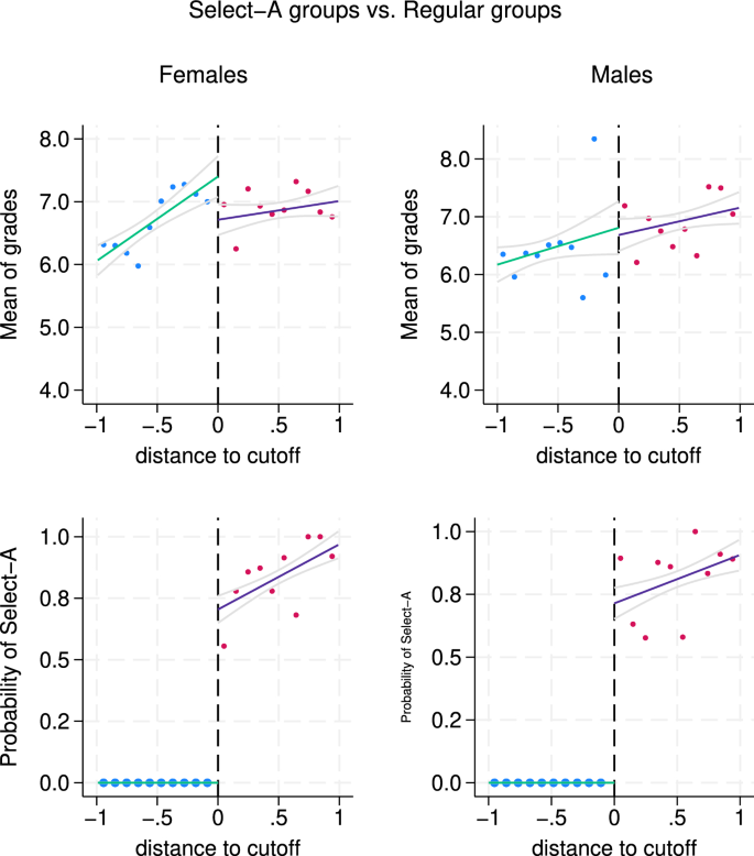
Jump in probability (first stage, bottom panels) and treatment effects (upper panels)

Full size image

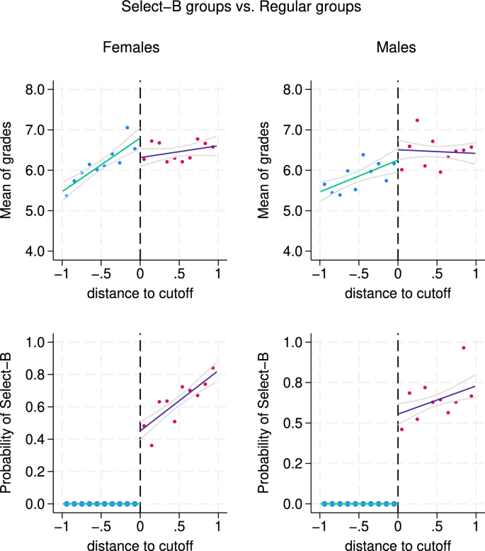
Jump in probability (first stage, bottom panels) and treatment effects (upper panels)

Full size image

In the bottom panels, the figures show a significant jump in the probability of treatment, joining a selective group, at the cutoff, and all observations with entrance scores below the cutoff remain in the regular groups. As anticipated, the probability of joining Select-B programme is appreciably lower, given the particular traits of this programme which require from students more than a high entrance score. The figure illustrates what is the main finding of this paper: there is a negative and significant jump at the threshold for the female sample, while the jump is non-significant, either being a positive or a small negative jump, for the male sample. Next, I provide further results as well as the numerical details on the estimated values and their levels of significance.

3.2 Baseline results

Table 3 displays the fuzzy RD estimates that corresponds to all grades pooled across common subjects. In the table, I show the results of the bias-corrected and robust nonparametric estimation for fuzzy RD proposed by Calonico et al. (2014a) and Calonico et al. (2014b).^Footnote11

A first finding to notice is the presence of gender differences in the first stage of the estimation—specifically, the probability of joining a selective group after surpassing the entrance cutoff. Males are somewhat more likely than females to enter selective groups, which may suggest that, as documented in the literature on gender differences in competitiveness, men feel more comfortable in competitive environments. This interpretation aligns, to a large extent, with the rationale I propose for gender differences at the threshold, as I will discuss below.^Footnote12

For the whole sample, if it were not split by gender, the result would be a negligible and non-significant treatment effect of 0.089 (on the 1 to 10 scale of the GPA) in Select-A groups and a non significant negative effect of 0.136 points in Select-B groups. This would lead us to conclude that high-ability groupings do not affect students’ performance, just as some many other studies have concluded (for instance, Abdulkadiroğlu et al. (2014) and Bui et al. (2014)). However, as in the figures above, the RD estimated effects provided in Table 3 show that there is a clear difference between females and males at the threshold. For males, I find either positive effects in Select-A groups or much smaller negative effects in Select-B groups; however, these estimates are not statistically significant in any case. The negative difference for females is around 1.2 points and 0.8 points in Select-A and Select-B groups, respectively, while for men the difference is either a premium of around 0.7 points or a penalty of around 0.1, still non-significant in both cases, at the threshold. The difference in the female sample is sizeable: if the average top female student in the regular group gets an average GPA of 9 over the year, their counterpart in selective groups obtains a GPA around or below 8. One first conclusion from these results is that neglected gender differences in selective environments can possibly be among the reasons why previous works have not found significant effects of selective academic programmes.^Footnote13

This difference in the performance of female and male students at the threshold is the key finding in this paper. A positive sign of the estimated treatment effects would be indicative of selective groups exerting a positive effect on performance, which could be a result, for example, of the interaction with smart peers or the higher quality of the classes in these groups. On the contrary, a negative jump in academic grades could be easily understood as a result of the higher difficulty and more demanding standards of selective groups. As a result of the positive and negative effects, negligible and/or non-significant results would also be possible. However, what is puzzling is why, whatever the advantages and disadvantages of selective environments are, the impact differs so clearly by gender. The results in Section 5 below will show that there are large gender-based differences on the response of low ranked students in selective groups that explains the observed jumps at the cutoff.

3.3 Heterogeneity of results across subjects

Heterogeneous effects could appear across different categories of subjects due to their specific, differential traits. To ascertain whether the RD results differ depending on the nature of the subjects, I separately consider three categories, or subfields, of subjects: economics-related subjects, business-related subjects and maths-related subjects.

Three main differences between these subfields might trigger gender differences in performance. First, the workload and the degree of difficulty of the subjects may differ by subfield (typically, students find mathematical methods and more analytical subjects to be more difficult). This could drive gender differences if women and men react differently to heavier workloads or greater difficulty.^Footnote14 Second, the degree of active participation in classes can differ by type of subject. For example, in business classes, the sessions are more frequently organized around teamwork and oral and group presentations in class time. This closer interaction among students through their teamwork can also reinforce the self-concept that each student holds in relative terms to their peers. Also possibly, the public presentations in front of other classmates may affect gender differences in performance if females/males tend to suffer different degrees of pressure in such type of situations.^Footnote15 Finally, the widespread stereotype that male students outperform female students in maths could reinforce gender differences in maths-related subjects.^Footnote16

Table 4 displays the RD results by subfield. Overall, in all three cases the results confirm the underperformance of female students and the overperformance of male students in selective groups with respect to their counterparts in regular groups. However, some differences appear across subfields. In economics-related subjects, the estimated effects are far from significant in all the cases, leading then to inconclusive results in these cases, both for males and for females. In business-related subjects and maths-related subjects, the estimated effects largely confirm the gender differences found in Table 3. In the case of business-related subjects, the negative jump in the female sample range from near 1 point in Select-A groups to around 2 points in Select-B groups. In this latter type of groups, the estimated effect for business subjects, though not significant, is negative and sizeable for male students too.

The effects in maths are also sizeable in the two types of selective groups, and the differences by gender are even greater. In Select-A groups, female students are near 2 points below their counterparts in regular groups, while male students exhibit a positive, large (1.13 points), and marginally significant differential. That is, males seem to perform relatively better in maths subjects once into selective groups. As a result, in these selective groups the gender gap in maths is the largest among all three categories of subjects. In Select-B groups the negative and statistically significant jump in the female sample is confirmed, though smaller (1.26 points), and again the estimate for males is positive (and above 1 point), though not statistically significant in this case. The stereotype threat hypothesis in maths, a field that tends to be competitive by itself, combined with the higher degree of competitiveness in selective groups, could well be explaining these large differences. Those students more negatively affected by competitive pressure, possibly females (Gneezy et al. 2003; Niederle and Vesterlund 2007), would tend to underperform more markedly. The overperformance of males in selective groups with respect to their counterparts in regular groups could be suggesting that, instead, males feel more motivated to exert effort in competitive environments.

Summing up, the RD estimated effects exhibit some heterogeneity by subfields. The gender differences are less clear in economics-related subjects but quite marked in business and, particularly, in maths. However, in all cases the gender differences point in the same direction, namely, a clear underperformance of females in selective groups with respect to women in regular groups, whereas no evidence of such effects is found for males, or, if any, positive.

Next, I perform several checks of validity for the RD design and results. The objective is to discard confounding effects, other that peer and/or rank effects, at the threshold. For the sake of exposition and to save space, in most of the cases I briefly refer to the check being made and results are provided in the Appendix.^Footnote17

The key identification assumption of the RD strategy is the continuity of the outcome variable at the threshold in the absence of treatment. Several conditions are taken as a guarantee of such continuity: no manipulation of the running variable, balance of sample characteristics that might impact the outcomes at either side of the cutoff, no jumps in the relationship between outcomes and the running variable in the absence of treatment, and no endogenous selection into the treatment group. In other words, for the RD design to be a valid strategy, the jump in outcomes at the threshold should neither respond to confounding factors occurring at that threshold, nor be a chance case where a jump in the relationship occurs.

In this paper, I emphasize the fact that important differences in rank ineluctably occur at the threshold and, thus, individuals in its neighbourhood are necessarily different in this dimension. This implies that even if all usual validity checks are passed, it still remains the doubt if what we are identifying is the standard peer effect, or the rank effect, or a mixture of both. I take then all the validity checks that follow as evidence to discard differences other than rank. Then, I proceed to analyse differences in performance across ranks of the ability distribution to the left and to the right of the threshold.

4.1 Manipulative sorting around the cutoff

Manipulative sorting refers to the possibility that agents can precisely control the assignment score to fall on the beneficial side of the cutoff. Such sorting of individuals would create a bunching of units around the cutoff. A discontinuity in the density near the cutoff is taken as evidence of such behaviour, and it is believed to invalidate the RD assumptions. Further, I would need to observe clearly different sorting behaviour by gender to infer that this might be driving the gender differences found with the RD results.

To check for the absence of manipulative behaviour, I formally test for sorting in my data using the proposal by Cattaneo et al. (2020). In particular, I use their robust bias-correction approach which uses bandwidth selection methods based on asymptotic mean-squared error (MSE) minimization.^Footnote18 The numerical results of the tests are displayed below each panel in Fig. 3, which also depicts the distribution of the running variable in all the three types of groups and by gender. The null hypothesis of the test is continuity of the density of the running variable (entrance scores) at the cutoff point. Both the test statistics and their p-values lead in all the cases to not reject the null of continuity in the density of the running variable.

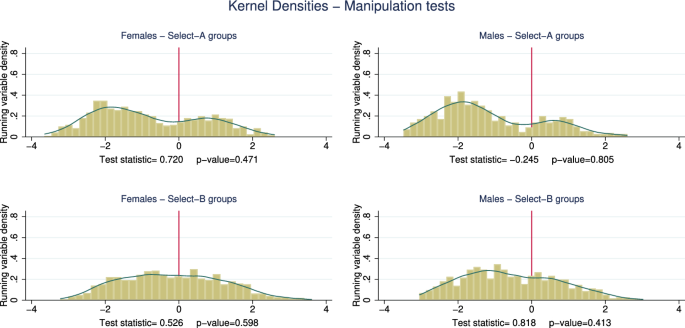
Density continuity/manipulation tests (Cattaneo et al. 2020). Regular groups vs. Selective groups

Full size image

4.2 Balance of students’ characteristics

To ensure that group assignments are the only source of discontinuity in the sample, we must check whether any other student characteristics potentially affecting GPA differ at the threshold. More importantly for my analysis, I must confirm that these differences at the threshold do not vary by gender.

Parental socioeconomic status (SES) is one of the key factors that can significantly impact students’ academic performance. Table 5 shows the estimated differences in the SES index around the threshold, as well as the differences in the proportion of students living at their parental home while attending university.^Footnote19 On average, students in the selective groups have higher SES than those in the regular groups. The difference is modest, approximately 0.5 points on the SES index’s 1-to-4 scale for Select-A groups and 0.35 for Select-B groups. Importantly for the sake of my analysis, the observed jumps in SES at the threshold do not significantly differ by gender. For the living-at-home indicator, the constant shows that over 80% of students live at their parental home while attending university. The only difference observed is a moderately higher proportion of female students in the Select-B group who live at home.

The higher SES of students choosing selective groups can be considered a stylized fact of these types of groups, as confirmed by the evidence for other countries (Campbell et al. 2020; Houng and Ryan 2018). This fact is undeniable, but the key question here is to what extent these differences in the SES index—and on the indicator of living at home—explain the jumps observed at the threshold and how these jumps vary by gender. On the one hand, as noted earlier, no significant differences are observed in the SES indicator between male and female students. On top of that, I provide evidence in Table 9 in the Appendix, demonstrating that the main RD results remain robust when using a balanced sample based on students’ socioeconomic status (SES) and the proportion of students living at home. Specifically, I trim the sample by excluding students in the lowest 25% of the SES index distribution within the regular groups and include only students who live at home. This trimmed sample shows no significant differences in the SES index across groups, nor any within-group differences between males and females around the threshold.^Footnote20 The RD jumps previously obtained, both in magnitude and statistical significance, largely hold across all cases. This provides further evidence that the differences in academic performance around the cutoff cannot be attributed to socioeconomic differences or to whether students live at home.

4.3 Placebo tests: jumps at artificial cutoffs

In the absence of treatment, jumps in the relationship between academic grades and entrance scores should not systematically occur. If they did, it would cast doubt on whether the jump at the threshold is a chance finding. To check for this, I perform placebo tests consisting of RD regressions at artificial cutoffs set at the 50th-quantile (the median) within each type of group.^Footnote21 Table 7 shows the estimated jumps for regular groups and for selective groups. Only 1 out of the 24 point estimates provided (i.e. 4.16 of cases) shows a significant jump, and this is the case of females’ GPA in Select-B groups when all subjects are pooled. This jump is not significantly found again when estimating by subfields, and it is of the opposite sign to the negative ones found repeatedly in the main RD estimations of Tables 3 and 4. Thus, I discard the possibility that the main RD results reported in Section 3 are chance findings.

4.4 Self-selection of students into selective groups

Enrolment in selective groups at university is voluntary, meaning that not all eligible individuals end up applying to such groups. This introduces an additional concern in the fuzzy RD design, since endogenous selection of individuals into the treatment groups might potentially bias the results. Ideally, we would like to observe into the regular groups all those applicants to selective groups who did not make it to be admitted, since this would further guarantee the comparability among threshold students.

For the estimation sample used in this paper, I lack information on the students’ choices beyond the observation of the group where they finally got enrolled. In the absence of data on applications of these students, I obtained access to the application forms fulfilled by students at UV in year 2013 and in the following four out-of-sample years, in total from 2013 to 2017. The admissions cutoffs for the two selective programmes have slightly increased with respect to year 2013, but the difference between them has remained at around 0.5 points as it was on average over the estimation period 2010-2013.^Footnote22 In these applications, which correspond to all students enrolling in any of the more than 70 major degrees offered by UV (around 9,000 students per year), students are asked to order their preferences for different degrees. The choice is conditional on students knowing their entrance grades, as students make their university applications after the entrance grades are published. They also know the approximate cutoff of each selective programme. This implies that only those who are not far away from the admission cutoff each year would be expected to apply formally for the selective programme. But conditional on this, that is, among those with an entrance grade sufficiently high, I can elicit the students’ preferences for joining one of the two selective groups used here, Select-A and Select-B groups, and also the major degree where those students who were not admitted into selective groups ended up enrolled.

The out-of-sample data contain, as in the estimation sample used in this paper, the entrance score of each student and the variables about the students’ socioeconomic background, students’ residence, and gender. I do not count, however, on academic grades once into the university. I neither have the information on the final destiny of those who might have applied for a degree at UV, and finally chose to enrol in any other university. This last percentage of people is expected to be near to negligible in the case of the selective programmes of business at UV, since, as above mentioned, the mobility of students to other regions is very low, the UV is the most prestigious among those around the region, and finally because there no exist other high-ability programmes in the region competing with the Select-A and Select-B programmes offered by UV.

According to the out-of-sample applications data, 989 students had as their most preferred option Select-A programme during the period, and 45.2 of these made it to be finally admitted into this programme. Among those who did not make it to enter, 48.3 entered into the Law degree offered by the UV, 40.01 chose the regular programme of business administration (the control group), and only 1.29 entered into Select-B programme.^Footnote23 These figures reveal, on the one hand, that the percentage of students not entering the Select-A programme who end up in the Select-B programme is very low. This confirms that students perceive Select-A and Select-B programmes as two differentiated options, and that the latter is not the preferred alternative for those not selected into the former. For instance, as mentioned in Section 2, students choosing the Select-A programme are likely to be avoiding the years of study abroad of the Select-B programme or the language requirements. On the other hand, students in Select-A likely share an interest for Law and BA, while students in Select-B groups are not likely inclined towards studying Law. A second implication is that those who did not make it to enter into Select-A groups are not finally enrolled into Select-B groups. Thus, rejected applicants to both Select-A and Select-B groups fill the regular groups of BA.

Another concern regarding the gender differences at the cutoff with the Select-A sample is the possibility that females/males had a more/less pronounced preference for Law/BA disciplines, which would imply motivational gender-based differences for studying BA subjects. If this were the case, the Select-B sample would not render comparable gender differences in the estimated jumps at the threshold. To investigate further that possibility, I estimate for applicants not admitted into Select-A programme, the probability of choosing finally the Law major against a BA major at UV as a function of the student’s gender, entrance score, SES index, and home residence, plus a set of year cohort dummies. The coefficient on the female indicator variable in that regression is 0.048, with p-value equal to 0.219. If no covariates are included, the unconditional gender difference is 0.034 with p-value equal to 0.460. These results show that there are not significant gender differences in such a preference for one or another discipline. This indicates that females enjoying less than males in the study of BA is not a plausible explanation of the gender differences in the RD jumps presented above with the Select-A sample.

As regards Select-B programme, it was the most preferred option for 1,163 students over the period 2013–2017, with 53.31 of them being finally admitted into the programme. Among those who did not make it to enter, 84.22 entered into the regular programme of Business Administration, 4.6 finally chose the Law major, and the rest chose either Economics or Finance & Accounting, both with lower admission cutoffs than the regular BA programme. The out-of-sample applicants data thus suggest that the bulk of students not being admitted into selective groups end up into the regular groups of BA.

4.5 Further evidence on differences in self-selection by gender

The literature documenting that women enjoy competition to a lesser extent that men do (Gneezy et al. 2003; Niederle and Vesterlund 2007) would suggest that, in order to avoid competition, high-performing women could be more prone than men to self-select into regular groups even when they pass the cutoff. These observations would not directly affect the RD estimation: since the RD methodology relies on individuals who are comparable in terms of their entrance scores, if students who passed the admission cutoff with a large margin decided to remain in the regular groups, they would not enter into the effective sample around the threshold used in the RD method. However, one potential concern is that a gender imbalance in the percentage of high-ability female students in regular groups could lead, through peer effects, to gender differences in the motivation and performance of their classmates, that is, in observations that enter the effective estimation sample used around the cutoff.

Two pieces of evidence would be indicative of such disparities in self-selection by gender: i) first, women with high entrance scores would appear appreciably more frequently than men in the upper end of the entry grades distribution in the regular groups; and, ii) second, the entrance score differential between the upper end of the distribution in the regular groups and the adjacent lower end of the distribution in selective groups would be higher for women than for men.

Fig. 4 and Table 6 provide evidence in this regard. In the upper half of the figure, I compare the densities of the entrance scores of females and males in regular groups (left-side panel) and in selective groups (the two right-side panels); in the bottom half of the figure, I compare the densities of the entrance scores of regular groups and selective groups for females (left-side panel) and for males (right-side panel). The upper plots show an almost complete overlap in the densities of males’ and females’ entrance scores within a group, particularly in the regular groups where they are almost identical. In addition, the proportion of students in regular groups that surpass the admission cutoff (in the bottom panels, the part of the regular group densities that lies below the densities of the selective group) is comparable for females and males. To be precise, the females’ entrance score density in regular groups shows a nonzero tail for entrance scores above 12.5 that is absent for men, but the proportion is so small that I rule out these differences as important enough to drive my results in regular groups. More formally, a Kolmogorov–Smirnov test of equality of distributions between females and males for the upper part of these distributions provides strong evidence in favour of the null hypothesis of equal distributions: the test values are of 0.094 with p-value equal to 0.726 for entrance scores above 10, and of 0.888 with p-value equal to 0.155 for entrance scores above 12.

Additionally, Table 6 allows us to compare the average entrance scores by gender at the upper end (deciles 9 and 10) and at the lower end (deciles 1 and 2) of the distribution in the regular and selective groups, respectively. For both females and males, the average difference is close to 0.5 grade points between Select-A group and regular groups, whereas this difference is almost null between Select-B and regular groups both for females and males. This further indicates that regular groups are not substantially more populated by high-ability females than high-ability males in the upper part of the distribution.

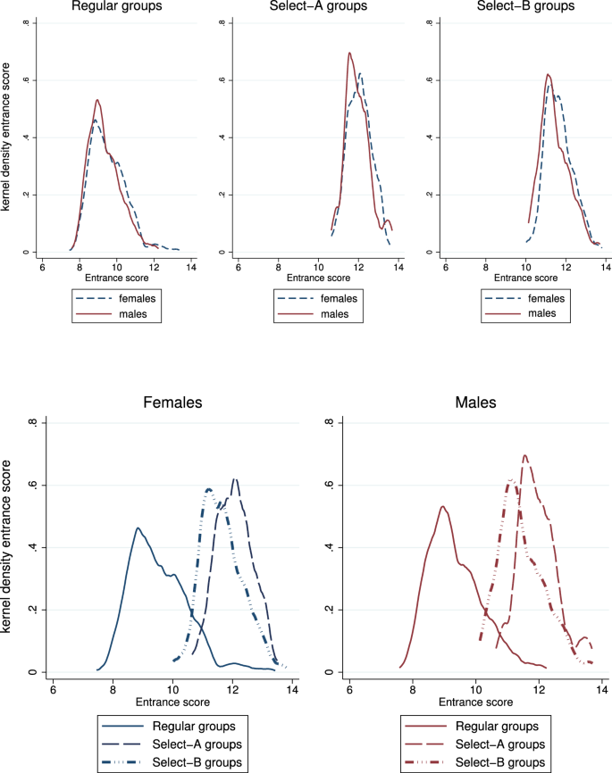
Kernel density of the entrance scores, by type of groups and gender. The graphs show the distribution across deciles of the final GPA distribution of those students ranked as decil 1 students according to the distribution of the entrance score

Full size image

After discarding other potential confounding factors at the threshold, in the next section I explore one of the main mechanisms through which entering a selective group can affect students’ performance: marginal students in selective groups are surrounded by peers in the classroom who are stronger than they themselves are. Different responses by gender to their resulting low position in the ability ranking could explain the RD jumps reported above, and this is what I explore next.

A general feature of selective settings is that they draw high-ability individuals from the global distribution of ability, thus creating a local (or within-group) distribution that modifies the rank position of each individual. The differences between the global and the local rank are less likely to affect those individuals in the upper and the lower ends of the global distribution: top ranked students in the global distribution are most likely at the top of the ability distribution within the selective group, and the lowest ranked students in the global distribution remain at the lowest end in their local one. However, the variation in rank is large at medium-high positions of the global distribution. This is particularly clear for students near the admission cutoff into selective groups: those who just made it into selective groups may change from intermediate/top positions in the global ability distribution to the lowest end of the local distribution in the selected group; those who end up allocated to the regular group become the top students of that group.

This idea is illustrated in Fig. 5, which shows the variation in students’ position in the ranking when comparing the global and local distributions of the entrance score. The graph illustrates that students who rank high in the global distribution may end up near the bottom of the ranking of the selective group after the selection criterion is applied. The vertical lines point out the entry cutoffs into the two selective groups, and permit to see that the downgrading of rank position of marginal students in selective groups is larger for Select-A groups, that is, the higher the admission cutoff is. On the contrary, students in the regular groups improve their ranking as a result of the truncation in the entry grade distribution caused by the selection criterion. (They lay above the 45 line.)

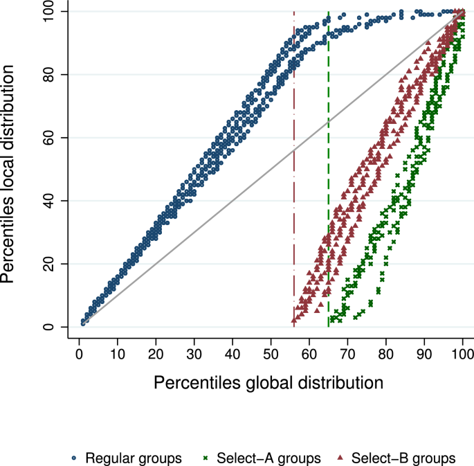
Ranking variation when comparing the global distribution to the local distribution of the entrance score. This graph illustrates that students who would rank highly in the global distribution may end up near the bottom of the ranking of the selective group after the selection criterion is applied. On the contrary, students in the regular groups improve their ranking as a result of the truncation in the entry grade distribution caused by the selection criterion (they lay above 45 line). The vertical lines point out the entry cutoffs into the two selective groups

Full size image

Do the patterns of students’ responses to the rank position differ by gender? To answer this question, we need to estimate differences in academic performance across students’ different rank positions controlling for the absolute ability of students. I proceed as follows.^Footnote24 I cut the entrance score distribution within each type of group and cohort (the local distribution) into deciles and rank students according to the decile they occupy. This local decile rank measure allows me to compare students ranked at the top and bottom with those ranked in the middle within a group. The main interest is to observe and compare the highest deciles in regular groups with the lowest deciles in selective groups since these are the students that compose the RD estimation sample. More specifically, the threshold sample used by the RD estimation in Table 3 is 100 composed of students ranked in deciles 8 to 10 in the regular groups, and 97 and 90 composed of students in deciles 1 to 3 in Select-A groups and in Select-B groups, respectively. To estimate differences in academic performance across the deciles I specify the following regression where I leave out as reference the 5th and 6th deciles and estimate the rank penalty/premium for the four lowest and four highest deciles within each group. The regression is run separately for the regular groups and for each of the selective groups, and by gender:

In equation (1),  stands for the GPA of student i of cohort c in module (subject) m;  is a binary indicator variable equal to 1 for students in the ith decile, with i varying from the 1st to the 4th deciles of their within-group and cohort local distribution, and equal to 0 in the rest of deciles; likewise,  is a binary indicator equal to 1 for deciles 7th to 10th and equal to 0 if otherwise;  is a second-order polynomial on the student’ cardinal entrance score^Footnote25;  is the student’s SES index; and  stands for a full set of module-cohort fixed effects; finally,  is the error term of the equation. To account for correlation among observations of a same module and cohort, standard errors are clustered at the module-cohort level.

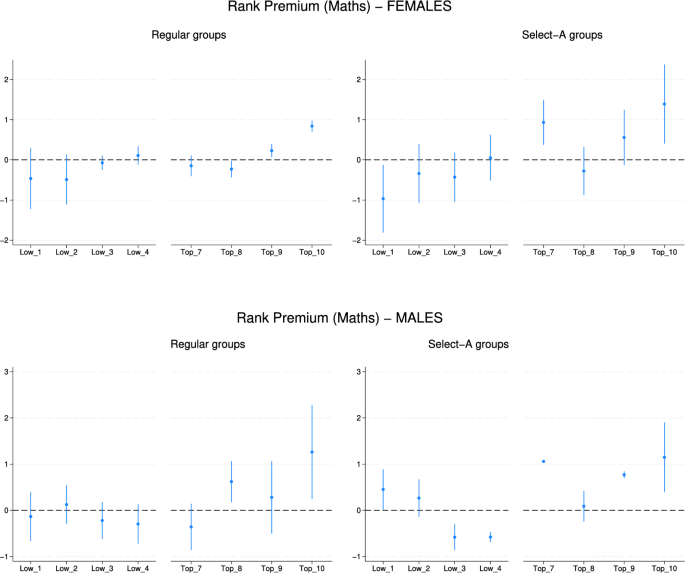
For brevity, I focus on discussing the rank effects estimated for maths-related subjects, as shown in Table 8. Results for the other three cases—all subjects, economics, and business—are available in the Appendix (Tables 10 to 12). I focus on maths-related subjects here because the gender differences in the RD results are the most pronounced in those cases. In all four tables, columns 1 to 3 show the results for females in all three types of groups, that is, in regular, Select-A and Select-B groups, respectively; columns 3 to 6 do so for the male sample. To explain the RD results in the neighbourhood of the cutoff, we need to compare the top ranked students in regular groups with the low ranked students in selective groups. In all type of subjects, top ranked students in regular groups exhibit positive, sizeable and significant rank premiums in regular groups (columns 1 and 4). In the case of maths-related subjects in Table 8, the estimated effect size for the top decile in regular groups is over 0.8 points on the 0-to-10 GPA scale for females and nearly 1.3 points for males.

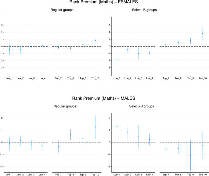
The positive rank premium found at the top of the regular groups’ distribution is in contrast with the rank effects at the lowest end of the distribution in selective groups and, more in particular, with the gender-based differences in such low positions. Female students at this lowest end show sizeable and significant negative rank effects both in Select-A and in Select-B groups. Contrarily, the results render a positive and statistically significant rank effect for male students in the lowest end of the distribution in both selective groups. In both positive and negative cases, the effects are larger in magnitude within the Select-B group—the most competitive of the groups. The positive/negative effects for the male/female samples hold their sign in decile 2 (although it is non significant for males in Select-A groups). Notably, negative effects for low ranked students appear in the regular groups for both female and male students, though these effects are smaller in magnitude and not statistically significant. This suggests that male students ranked lowest in the selective groups are particularly motivated to improve their standing, an effect not observed among female students or males in regular groups. Conversely, while low ranked female students tend to underperform across all group types, this pattern is especially pronounced in selective groups, and even more so in the highly competitive Select-B group.

Tables 10, 11 and 12 in the Appendix present some heterogeneity in the estimated effects by subfields. However, the gender differences in the lowest deciles of selective groups remain pronounced: female students in the lowest deciles significantly underperform, while males do not show this behaviour. The strong performance of top students in regular groups is also consistent across all cases.

The conclusion is that upon entry into a selective group both female and male students face the opportunity cost of giving up to a top position in a regular group, what would in principle suggest negative jumps at the threshold for both genders. However, the results highlight noticeable gender differences in the behavioural response of male and female students that find themselves as the lowest ranked students in selective groups. The stronger rank effects in maths-related subjects help explain the relative larger gender differences of the estimated RD jumps found for type of subjects.

To visualize these sharp contrasts at the threshold, Figs. 6 and 7 display the estimated rank effects in maths-related subjects. Fig. 6 compares the estimated rank premium in regular groups (left panels) with Select-A group (right panels), both for females (upper part of the graph) and for males (bottom part). Fig. 7 illustrates the results for Select-B group. Overall, the figures reveal that the most striking differences are between female and male students in the lower deciles of selective groups. In the case of Select-A groups in Fig. 6, as long as we move towards the upper part of the distribution the results show fewer differences by gender. In other words, at the top of the distribution of ability, there are not so marked differences in the responses by gender within a same type of group, at least with regard to the sign of such responses. Both males and females overperform in the top positions in Select-A groups. In Select-B groups, as shown in Fig. 7 a somewhat different pattern shows up in the male sample, with students in top positions not exhibiting significant overperformance with respect to the intermediate deciles—if any, the effects are negative, although the estimated errors are large and the effects are not found to be significant.

I draw three conclusions from these findings. The first one is that, after discarding other mechanisms and potential confounding effects at the threshold, the rank effects, and the differences by gender that they exhibit, become the most likely explanation for the obtained RD results. The second is that the gender differences found in the RD jumps respond to the different behaviour of male and female students who are low ranked in selective groups. While males seem to respond very competitively in selective groups, probably trying to avoid the stigma of remaining in low positions of the ranking, females do not seem able to exert such positive response in the lowest positions and reveal themselves as affected by a small-fish-in-a-big-pond effect that leads them to underperform markedly at the threshold. A third conclusion is that the different degrees of competitiveness of the different groups seem to affect the response of students’ to their relative standing in the group.

These results find general support in the recent contributions documenting the role of ordinal rank and relative standing of individuals in a group as an additional determinant of performance. Overall, in regular groups, the pattern observed would be that of a positive rank effect, both among females and males. These results line up with the findings of the recent literature on rank effects, which have firmly documented a positive rank premium (Murphy and Weinhardt 2020; Elsner et al. 2021).

This literature, though, has devoted less attention to the shape of these effects over the distribution, or it has largely found homogeneous effects (e.g. Murphy and Weinhardt (2020)). However, my results point to differences in rank effects depending on the degree of selectivity of the group. The large underperformance of female students ranking low suggests that female students who view themselves as the small-fish-in-a-big-pond in a selective environment find it more difficult than their male classmates to neutralize the negative impacts of the downgrading in terms of ranking that the new situation entails. A notable erosion of their self-confidence in these groups is one of the possible explanations.^Footnote26 Importantly, within a same type of group, my results do not show so remarkable gender differences in rank effects in the top positions. Thus, the hypothesis that females are more likely to chock under pressure than men do in competitive environments seems quite less clear when their rank endows them with high self-consciousness.^Footnote27

In my results, the positive response of male students in low positions is specific to selective groups. That higher levels of competitiveness may trigger different behavioural responses to own relative standing is addressed by Azmat et al. (2019).

The authors show that, in a context where individuals have competitive preferences, learning that one’s relative ability is lower than initially believed leads to greater exertion of effort. Low ranked individuals in selective groups experience a similar ’surprise’ in rank position, since their rank in the local distribution within the selective group is in sharp contrast to their top position when at high school, prior to their entry to university. Given the high competitive pressure in selective groups and the documented higher preference for competitiveness of males (Andersen et al. 2013; Sutter and Glätzle-Rützler 2015; Niederle and Vesterlund 2007), it follows that males would be predicted to exert more effort when low ranked in selective groups.

The last-place-aversion hypothesis of Kuziemko et al. (2014) also provides an explanation for a motivated behaviour of very low ranked individuals. These authors explore the shape of the ordinal rank effects depending on the position of individuals in the distribution and find, in their words, that individuals exhibit a particular aversion to being in last place, and that a potential drop in rank creates the greatest disutility for those already near the bottom of the distribution (p.106).

This can also explain the positive response of the lowest ranked males in selective groups, who would exert extra effort in order to avoid the stigma of being at the last positions. The contrast with the prior high-rank position when in high school could exacerbate this feeling.

The gender differences found among low ranked individuals in selective groups may have important consequences on the subsequent gender differences in behaviour and performance within such selective groups and, ultimately, once into the labour market. Those unable to escape from the lowest positions may have their self-esteem permanently undermined in these groups. In cases such as Select-B groups, an immediate consequence of being stuck to the last positions is the loss of opportunities in the auctions for choosing a university abroad under the UV exchange programme.^Footnote28 It follows that at the lowest positions, those affected by last-place aversion will tend to move towards higher positions of the distribution of performance, while under the small-fish-in-a-big-pond effect the lowest positions will tend to perpetuate. As a piece of evidence in this direction, I show in Fig. 8 kernel densities of students’ GPA-based deciles at the end of their first year at university for those who were ranked initially the lowest (decil 1, left panels) and the top (decile 10, right panels) according to their entrance grades distribution. The graph illustrates that, in selective groups, male students who were initially low ranked tend to move up over the GPA distribution to a larger extent than females do in these groups, while this gender difference is not evident in regular groups.

Rank Premium. Regular groups vs. Select-A groups

Full size image

Rank Premium. Regular groups vs. Select-B groups

Full size image

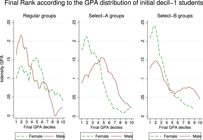
Rank change for students initially low ranked as decile1. This graph shows the kernel densities of students’ GPA-based deciles at the end of the first year at university for students who were ranked initially the lowest according to the entrance grades distribution. In selective groups, male students who are initially low ranked tend to move up over the GPA distribution to a larger extent than females do in these groups, while this gender difference reverses in regular groups

Full size image

This paper examines gender differences in academic performance among students barely entering selective university groups. Using administrative data from business students in both selective and regular groups, I apply a regression discontinuity design to compare GPA performance in common subjects during the first academic year. I find large, significant negative drops in GPA at the cutoff for female students in selective groups, while male students show either small and insignificant changes or even positive jumps.

After ruling out other potential mechanisms influencing academic outcomes near the entrance threshold, I analyse performance differences by position in the ability distribution within each group, conditional on absolute ability. My results suggest a substantial opportunity cost for students who barely qualify for selective groups, as they forgo top positions in regular groups. However, the net effects differ by gender. Males in the lowest positions of selective groups tend to exert more effort, likely to escape these positions, whereas low ranked female students typically show a marked underperformance in selective groups as compared to their peers in the middle deciles.

This evidence suggests that rank effects can spoil the otherwise positive effects from joining better peers. The effect is particularly damaging for female students who find it more difficult than their male classmates to neutralize the negative impacts of the downgrading in terms of ranking and the higher competitiveness that the new situation entails. Importantly, within a same type of group, my results do not show so remarkable gender differences in rank effects in the top positions. Thus, the hypothesis that females are more likely to chock under pressure than men do in competitive environments seems quite less clear when their rank endows them with high self-consciousness.

Beyond gender implications, my results suggest that selective grouping based on ability can have several implications for economic decision-making, human capital formation, and education policy. i) For individuals deciding whether to join a selective group, the opportunity cost is the academic premium associated with holding a prominent position in less demanding environments. In academia, particularly in higher education, this may reduce the chances of success in postgraduate applications, scholarships, or job offers when competing with candidates from standard programmes based on academic records. My results underscore the need for postgraduate selection processes to consider university performance relative to the type of programme completed. ii) Admission score thresholds in selective programmes can create a potentially harmful distortion in the information about individuals’ absolute abilities. This could have two further implications for human capital formation. First, it might prevent future employers from recognizing the best-prepared candidates in processes where academic records are crucial. Second, it could undermine the individual’s confidence in their academic abilities, leading to suboptimal investments in human capital development. iii) From an education policy perspective, my work suggests that the additional resources often required for these special programmes may not be cost-effective if the expected effects are not achieved. Informational interventions within selective groups, such as emphasizing the importance of absolute ability over relative performance, could help reinforce academic self-esteem, especially for female students who may feel less comfortable in these settings.

I do not interpret my results as evidence against the value of high-achieving groups in education or other contexts, nor do I suggest that women avoid such groups. Interaction with motivated peers, preparation for demanding careers and the quality of teaching and learning are benefits of selective groups that go beyond academic grades. Further research is needed to explore whether these groups also foster an environment that prepares students for a competitive labour market.