Article Content
Abstract
We use a simple yet powerful approach to investigate the dynamics of worker flows across sectors in the Spanish economy. The method imposes a minimal amount of structure on the data by assuming sector-specific matching functions, and backs out the direction of workers’ search intensities across sectors using data on realised worker flows and vacancies. We find that aggregate search intensity in Spain has been increasing since the pandemic and has led aggregate labour shortages to be below pre-pandemic levels by 2023. However, this boost of search intensity is directed to industries with low matching efficiencies and job finding rates. As a result, aggregate match formation is near to a 10-years low relative to the number of matches that would result if search intensity was allocated to maximise total matches given the observed vacancy distribution and match efficiencies across sectors.
Explore related subjects
Discover the latest articles and news from researchers in related subjects, suggested using machine learning.
- Labor Movements
- Labour Law/Social Law
- Labor Economics
- Labor and Population Economics
- Sociology of the labour market
- Unemployment
1 Introduction
How do labour markets reallocate resources after aggregate and sectoral shocks? There has been renewed interest in answering this question in light of post-pandemic labour shortages. For example, the OECD 2024 Employment Outlook reports large labour shortages across its members immediately after the pandemic, with many economies still experiencing substantial labour shortages by the end of 2023 (OECD 2024). Although there are several ways to measure these shortages, the ratio of vacancies to unemployment has been repeatedly used to gauge their extent. This ratio, also known as labour market tightness, aims to capture the number of job positions searching for workers relative to the number of workers searching for these positions. It therefore assumes that the number of unemployed provides a good estimate of the number of workers searching in the economy.
By this measure labour shortages in Spain were at a 10-year high in 2023. Further, the OECD reports Spain to have the third largest level of labour shortages among European economies, only slightly behind Belgium and the Netherlands (OECD 2024). In light of this evidence, one might be tempted to argue that the duality of the Spanish labour market is helping generate persistent shortages, pushing workers away from precarious jobs in labour intensive industries. However, other economies with similar labour market structures like France and Portugal appear not to be facing major shortages, casting doubt on this explanation. In this paper, we investigate the roles labour demand and labour supply have been playing in generating shortages in Spain. The novelty of our approach is that we take into account worker reallocation across sectors and hence can shed light on whether shortages arise due to workers not searching in sectors with high job finding rates.
We use the sectoral search model developed in Carrillo-Tudela et al. (2024) to separately estimate the roles of labour demand, labour supply and matching efficiency in explaining the observed dynamics of sectoral labour flows and aggregate employment matches among employer switchers. Our model builds on the canonical Diamond-Mortensen-Pissarides (DMP) framework but divides the economy into different “islands” or sectors, each characterised by its own sector-specific matching function with sector-specific inputs and exhibiting a sector-specific matching efficiency parameter. Aside from the stock of vacancies being posted in a given sector s, we use total search intensity directed towards sector s as the second input in the sectoral matching function.
Search intensity in our model arises from workers searching in their own sector s and from workers searching in different sectors who target jobs in sector s. Furthermore, search intensity directed to a sector s is differentiated by whether the worker is employed, unemployed or inactive. In this environment the appropriate measure of labour shortages is then the vacancy-search intensity ratio instead of the standard vacancy-unemployment ratio. We argue that our measure better captures the extent to which workers are searching for open positions, as it takes into account that the employed and those in inactivity also search for open positions as well as the role of heterogeneity in search intensities by workers’ sector of origin and employment status.
To estimate our model we focus on mobility across industries and use the Spanish Labour Force Survey and the Labour Cost Survey between 2013 and 2023. A key advantage of our model is that it can be estimated only using data on the stock of employed workers in a given sector, the stocks of unemployed and inactive workers with a known last sector of employment, worker flows across sectors, and sector-specific vacancy stocks. To separately identify search intensities towards a given sector and that sector’s matching efficiency we follow Shimer (2004) and use information on the observed search activity among employed workers. Using the vacancy-search intensity ratio we show that labour shortages peaked around the start of the pandemic and by 2023 they were about 1.5 percentage points below this peak. We find that the decrease in labour shortages occurred across all industries. Although we measure less severe labour shortages relative to the standard measure, shortages remain high, in line with the conclusions of the OECD 2024 Employment Outlook.
The main result of the paper is to show that the persistently high labour shortages in Spain arise from workers directing much of their search intensity towards low matching efficiency and job finding rate industries. We compute the distribution of search intensities that maximise the total number of matches across industries. Carrillo-Tudela et al. (2024) label this the Match Maximising Allocation (MMA). The concept behind the MMA builds on Şahin et al. (2014), who measure the level of mismatch between searching workers and vacancies across sectors. However, instead of focusing on the efficient allocation of search intensities, our measure aims to maximise the number of matches taking as given the observed distribution of vacancies and estimated matching efficiencies.
We find that the Spanish labour market has been moving away from the search intensity allocation implied by the MMA and it is nearly at a 10-year low. The MMA exercise suggests that to reduce labour shortages the search intensity towards Construction needs to be 8 times larger than the search intensity we estimate in our benchmark model, while search intensity towards Other Services needs to be 8 times lower. This result arises as we estimate Construction to have the highest matching efficiency and job finding rate per unit of search efficiency, but Other Services to have one of the lowest values on these dimensions. This contrast reflects that in the LFS we observe three times more workers employed in Other Services declaring active job search relative to workers employed in Construction, while both industries exhibit similar amounts of worker reallocation. Further, these two industries stand out as the estimated search intensities towards the remaining industries are about the same as the ones implied by the MMA.
It is important to note that our exercise illustrates gains to reallocating search activity in terms of filling existing vacancies and maximising employment, assuming perfect substitutability across different skills. It does not suggest that this outcome is efficient or that we are advocating for workers to shift their search intensity towards Construction. Nevertheless, it poses the question of why Other Services exhibits one of the lowest matching efficiencies and job finding rates among all industries even though vacancy creation is similar in this sector as in other low-skilled sectors as Construction.
We also highlight that it is the distribution of search intensities across sectors and not the level of search intensities what appears to be causing high labour shortages in Spain. Indeed, our analysis shows that aggregate search intensity has been increasing since 2019, after many years of decline. The rise in search intensity occurred across all employment status categories, with employed and unemployed workers increasing their search intensities towards permanent contract jobs and unemployed and inactive workers increasing their search intensities towards temporary contract jobs. Further, search intensity has been the main driver behind the procyclicality of the gross mobility rate and the countercyclicality of the net mobility rate across industries. By means of counterfactuals we show that equalising search intensities across sectors at each point in time drastically reduces the cyclicality of gross mobility and net mobility, while equalising the stock of vacancies or matching efficiencies across sectors does not seem to have any meaningful effect on the cyclicality of gross or net mobility.
The second key result of the paper is that aggregate matching efficiency decreased since its peak in 2019, after many years of improvement, displaying the exact opposite pattern as that of search intensity. In a context of (mostly) rising labour demand, measured as the number of vacancy postings, we find that the aggregate job finding rate per unit of search intensity has also been decreasing since its 2019 peak across. Further, the deterioration of matching efficiency and job finding rates occurred across all industries. Thus, the main reason behind the observed rise in the number of new employment matches in Spain since the pandemic has been the rise in workers’ search intensity.Footnote1
The reduction in the industries matching efficiencies arises as we observe a relative moderate increase in workers’ employer-to-employer transition rates, but a strongly increasing measure of search effort among these workers. As a consequence the model explains this tension through a reduction in each industry job finding rate. With rising vacancy-search intensity ratios, each industry’s matching function then implies a decreasing matching efficiency. This result appears robust to different modelling strategies. We show that a decreasing (aggregate) matching efficiency also results when estimating the standard DMP model’s (aggregate) matching function on Spanish data.
Related literature:
This paper contributes to the growing literature investigating the causes of labour shortages. In particular, Costa Dias et al. (2021) develop a measure of labour market opportunities for UK workers using the historical occupation-to-occupation transition matrix. Essentially the current degree of opportunity for a worker in a given occupation is the number of vacancies posted in all occupations in the economy, weighted by the historical probability that similar workers transition to that occupation. Our approaches are conceptually very different, while both using historical transition matrices, as we back out a time-varying measure of the direction of worker search intensity while they use the average past transition matrix to study where workers tend to find work.
Additionally, our match maximising allocation exercise is similar in spirit to the notion of mismatch developed by Şahin et al. (2014) and applied to the UK in Patterson et al. (2016). While we abstract from a full model-based optimal policy, we extend their results to measure mismatch in our model with a rich data-driven notion of the labour supply received by each industry, where differences arise because we consider workers search intensity to be directed to jobs outside of their last industry.Footnote2
We also contribute to the literature which measures gross and net worker mobility across industries and occupations. Kambourov and Manovskii (2008) document rising worker mobility between 1968 and 1997 in the US. Carrillo-Tudela et al. (2016) investigate the level and cyclicality of mobility in the UK using the LFS data. Carrillo-Tudela et al. (2023) extend their findings to the Covid recession, and directly measure which industries and occupations workers are searching for jobs in using survey questions added to the Understanding Society dataset. Cortes et al. (2020) use labour market flows to investigate the drivers of the decline in routine jobs in the US. Faberman et al. (2021) measure search effort of employed and non-employed workers in the US using the Survey of Consumer Expectations. Relative to these papers, our contribution is to disentangle the role of worker search intensity and direction from firm vacancy posting patterns in driving reallocation across industries.
Finally, we contribute to the growing literature investigating the post-pandemic behaviour of the Spanish labour market. In particular, Diaz et al. (2024) and Busch et al. (2024), consider the effects of worker reallocation in a dual labour market setting. Our contribution is to measure the intensity of search across different sectors and show its behaviour towards temporary and permanent contracts. Further, our analysis provides an illustrative outcome of reallocating workers’ search in order to achieve the maximum number of employment matches in the Spanish economy. Our exercises suggests that search intensity needs to be allocated to sectors with high matching efficiencies and job finding rates (per unit of search intensity). Although the boom in the Construction sector severely affected the Spanish labour market, our findings reflect that, conditional on the distribution of vacancies observed during the post-pandemic period and the estimated distribution of matching efficiencies, Construction exhibits the highest job finding rate per unit of search intensity in the economy and hence offers searching workers one of the highest employment probabilities.
The remainder of the paper proceeds as follows. In Sect. 2, we introduces our theoretical framework and explain how to use it to separately identify search intensities by sector and employment status and sectoral matching efficiencies. Section 3 discusses the data and its limitations as well as presents the aggregate results from our estimation and its implications for sectoral reallocation. Section 4 revisits labour shortages in Spain and compares the sectoral direction of search intensities estimated by our model and the ones implied by the Mach Maximising Allocation. Section 5 concludes.
2 Framework
The objective is to separately estimate the roles of labour demand, labour supply and matching efficiency in explaining observed sectoral labour flows. To this aim we will use the framework developed in our companion paper Carrillo-Tudela et al. (2024), where we analyse the roles of these components in a cross-country setting. For completeness, here we present such a framework.
Consider an infinite-horizon economy that is divided into sectors , where S is the total number of sectors, and define a time period by Each sector is populated by workers and firms. Workers can be employed, unemployed or inactive. Let denote the stock of employed workers in sector s at time t, the stock of unemployed workers in sector s at time t, and denote the stock of inactive individuals in sector s at time t.Footnote3 Let denote the number of active vacancies in the sector.
Workers in our economy can find a new job in their own sector or in a different sector. Let denote the number of workers who were employed in sector s at time t, and who are employed in sector at time . Similarly, denotes the flow of workers who were unemployed at time t, whose last job was in sector s, and who are employed in sector at time . Finally, denotes the flow across sectors via inactivity in an analogous way. We define as the total number of new matches formed in sector at time . This is the sum of all new matches from employment, unemployment, and inactivity, arising from workers arriving from all sectors s:
The key assumption is that there is a sector-specific matching function that mediates the number of new matches in a given sector at time t. Specifically, for each sector
gives the number of new matches formed (between t and ) as the result of a constant returns to scale (CRS) matching function M(.). The inputs to this matching function are the total search intensity units directed towards sector , , and the number of vacancies posted in sector , . The parameter is the sector and time-specific match efficiency, and captures the effectiveness of matches due to, for example, sector-specific practices, technology, and firms’ recruitment strategies, among other dimensions, that we assume independent from workers’ search intensities.
Total search intensity arises from workers across employment status and sectors. In particular, let denote the search intensity units of employed workers in sector s towards vacancies posted in sector at time t. Similarly, and denote the search intensity units of unemployed and inactive workers, respectively, towards vacancies in sector . We assume that , and are exogenous and capture workers’ search effort, search direction and acceptance choices, as well as sectoral reallocation frictions (skill gaps, geographical mobility costs, etc). Aggregation implies that total search intensity directed towards sector is given by
Defining the sector-specific labour market tightness and using the CRS property of the matching function, the job finding rate per unit of search intensity in sector is given by . This implies that all workers searching for jobs within sector face the same congestion through a common . However, workers’ contribution to congestion depends on their search intensities, , and . The transition rates from sector s into employment in sector can then be expressed as
where is the rate at which workers employed in sector s in period t find new employment in sector in period , is the rate at which unemployed workers in sector s in period t find employment in sector in period and is the rate at which inactive workers in sector s in period t find employment in sector in period .
By summing over all sectors , we can express the corresponding transitions rates away from sector s into employment in other sectors as:
Note that since total search intensity can take any value, both the direction and total amount of search intensity can affect transitions rates. For example, for employed workers in sector s we can express the transition rate , where is their total search intensity and the term in brackets is the weighted average of the job finding rates per unit of search intensity in the sector these workers are search in.
Finally, we can define further aggregates by simply summing over all sectors. Total new matches formed in a given period are defined as , and total economy-wide search intensity is . The aggregates corresponding to vacancies and worker stocks are defined similarly as , , , and . The aggregate transition rates of each worker group are defined as expected. For example, with the aggregate UE rate given as , and aggregate vacancy filling rate as . Aggregate labour market tightness can be defined as . However, recall that there is no aggregate matching function, and so worker flows also depend on the allocation of vacancies and search intensities across sectors.
2.1 Identifying search intensities
For given parameters of the model, the search intensities, and the various market tightness, can be backed out using observed worker flow data. In particular, replacing in using (1), our framework implies sectoral flow rates , and can be expressed as:
Assuming that we have already estimated the matching efficiency parameters, , and know any other parameters such as the matching elasticities behind the matching function, then the above set of equations allow us to estimate search intensities , and for all pair from the observed transition rates. Specifically, at time t, data on (i) transitions rates across sectors, , , and , (ii) vacancies, , and (iii) worker stocks, , , and , imply that (3), (4), and (5) provide a system of equations in the unknown search intensities, . Under standard regulatory conditions on the matching function, a fixed point argument shows that the solution to this system of equations exists and gives a unique value for each search intensity.
Intuitively, the higher is a given observed transition rate from sector s to , for example , the higher the search intensity employed workers in sector s must have towards jobs in sector . This follows from rearranging (3) to give . This expression shows, however, that is mediated by two factors. Firstly, the job finding rate per unit of search intensity in sector . Secondly, there is an interaction effect as an increase in increases the total search intensity towards sector , which then crowds out search by endogenously lowering . This crowding out effect is one of the reasons that analysing our estimated search intensity adds value over just investigating the flows themselves.
Summing up the estimated search intensities yields the total search intensity directed towards each sector, , as defined in (1). This then immediately gives the estimate of market tightness in each sector as . The tightness estimate can also be understood more simply as being backed out directly from the observed vacancy filling rate: we can use the observed to invert to solve for . Recall that since the vacancy filling rate is calculated as new matches per vacancy, this also uses our worker flow data, and is just an equivalent way of interpreting how the equations above are solved. This simple identification of search intensity and its direction across sectors from the realised cross-sectoral flows in the economy forms one of the core steps of our framework.
2.2 Identifying matching efficiency
Equations (3), (4), and (5) make clear that identifying search intensities can be achieved as long as we know the matching function parameters. In this section, we discuss how to identify one key set of parameters: the matching efficiencies, . At each time t, there are only S of these match efficiencies, one per sector. The matching efficiencies control the size of the job finding rates , and hence allows us to separate the role of and search intensities . To identify we will leverage on the search effort measure proposed by Shimer (2004) and followed by Mukoyama et al. (2018) to analyse the cyclicality of unemployed workers’ search effort. We present the most general version of this approach and discuss the key intuitions. In our empirical application we will take a slightly more restricted approach in order to reduce the number of degrees of freedom in our estimation.
In European Labour Force Surveys individuals are asked whether they are actively looking for another job, even if they are currently employed. If they respond affirmatively, they are further asked about the search channels they have been using in their search. This information allows us to construct aggregate measures of search effort by computing the fraction of workers, among given defined groups, who declared themselves as active job searchers and weight each respondent by the fraction of search channels (among all possible search channels asked in the survey) they are using. Information on search channels allows us to capture each individual’s intensity of search. Specifically, let denote the number of employed workers in sector s who reported actively searching for a job at time t weighted by the proportion of search channels used (among all possible search channels asked in the survey).Footnote4 We let be our empirical measure of the total search effort among employed workers in sector s at time t.Footnote5 In our framework the total search intensity of employed workers in sector s equals the sum of these workers’ search intensities across all receiving sectors. The key identifying assumption is thus to impose
That is, variation in the search effort of employed workers across sectors and time help us identify variation in the job finding rates per unit of search intensity in the destination sectors given observed transitions rates . Notice that, at each time t, (6) adds S new equations to the model. Since we are trying to identify the S match efficiencies, , this offers a solution to identifying the match efficiency terms separately from the search intensities ones.
2.3 Estimation procedure
To estimate and we need to solve the set of nonlinear equations described in (3), (4), (5) and (6). In practice, we proceed as follow. Let and be column vectors containing the empirical measures of search efforts and the inverses of the job finding rates per unit of search intensity, respectively. Let denote the matrix of employed worker flow rates across sectors. Then we can stack the S equations in (6) to yield a matrix equation which allows us to solve for from
by taking one over all the elements of element-wise allows us to recover each . The key behind this procedure is that we are solving for the job finding rates of the receiving sectors (“what is the probability of finding a job in sector ?”) using data on how hard workers in each sending sector are searching (“how hard are workers in sector s searching?”). This is where the matrix inversion comes in, by using the realised employer-to-employer transition matrix to make a connection between all of the sectors. Intuitively, a sector s must have a high job finding rate if workers have a high overall employer-to-employer rate to sector s, but the sectors from which workers make these changes have a low total search effort (weighted according to the relative employer-to-employer rates from all sectors to sector s). This can be seen from the formula : the job finding rates are a weighted sum of the total search efforts , weighted by the employer-to-employer transition rates .Footnote6
Having estimated the , we can now back out the search intensities , , and by rearranging Eqs. (3), (4), and (5) such that , , and , for all . We then add up these search intensities to yield total search intensity towards each sector, , using (1), and market tightness in each sector, using . The final step is then to back out the matching efficiencies in each sector by inverting for each s. That is, we find the needed to explain the estimated given the estimated tightness.
Implementation: We follow the literature and assume a Cobb-Douglas matching function such that , where is the elasticity of the matching function with respect to . This implies that we need to also recover . To do this we separate the estimation into an inner and outer loop such that we follow the outlined estimation procedure for , , and in the inner loop for a fine grid of guess of . In practice, we restrict , such that each sector is described by a fixed effect and a common time-varying component. By time averaging the data and inverting to solve for from , and then using to match each period, we obtain a unique value for and find that the estimates of are unique in our numerical procedure. We then compute a time series for , implied by each guessed value of . We use these as data points and estimate as the minimiser of the standard deviation of . We choose this procedure by analogy with a simple OLS estimation of a matching function (e.g. , where ) which minimises the sum of squared residuals , which is equivalent to minimising the standard deviation of .
3 Application to the Spanish labour market
3.1 Data
We use two surveys to build the required data. The first one is the Spanish Labour Force Survey (LFS), which is the quarterly household survey that provides the official employment and unemployment measures for Spain and the source for EUROSTAT data. This survey is carried out by the National Statistics Institute (INE) and contains an average of 134,888 individuals per quarter during the 2005–2023 period. The survey is organised as a 6-quarter rotation panel, with stratified sampling and sampling weights. We use weighted observations throughout our analysis. Given the standardised nature of the LFS we use the ILO classification variable, information on the type of employment contracts and the self-employed indicator variable to classify workers into 5 groups: employed with an open-ended contract, employed with a temporary contract, self-employed, unemployed and inactive (out-of-the labour force).
For every quarter we aggregate up individuals to generate the stocks of workers across three employment status and ten 1-digit SIC (industry) groups: , , and . For a given quarter we assign the last or current industry where we observed the individual working as his/her sector s. We also use quarterly information to construct data on the fraction of employed workers who are actively searching by industry. To construct labour flows, we use the confidential, scientific use version of the LFS that includes a variable linking individuals across quarterly interviews. The key objects are the “current-state to employment (X2E) flows”, expressed as the rates , , and . Note that these rates are based on the flows from t to , and for workers non-employed at t we have information about their last industry of employment (s) even though they are not working at time t.
There are three sources of missing data that prevents us from fully capturing all transition flows: (i) workers who have been unemployed/inactive for more than a year, (ii) non-response in the survey, and (iii) new entrants into the labour force. The main concern for our estimates is the first reason, the length of non-employment. A common feature of European Labour Force surveys is that the previous industry or occupation of a non-employed worker is not known if the individual had jobless spell of more than one year. Nevertheless, for our methodology it is more important to know the destination rather than the origin of the workers. However, we acknowledge that the missing information will bias upwards our estimates of search intensity for unemployed and inactive individuals, as it will mostly reflect the search intensity of the short-term non-employed. We keep the long-term unemployed/inactive in our data, assigning them into a “long-term unemployment” category. The base estimation of search intensity includes these later group.Footnote7
Our second source of data is the Labour Cost Survey (Encuesta trimestral de costes laborales). This survey is also carried out by the INE and gives the unit labour cost estimates for Spain. Since 2013 the Labour Cost Survey (ETCL) includes a question about open vacancies in a firm. The survey is designed as a rotating panel where 20% of the firms rotate every quarter, with the exception of those firms larger than 500 workers, who are all sampled and followed. The survey covers around 28,000 firms every quarter that are chosen to give a representative sample of firms in Spain. Further, the survey provides a breakdown of vacancies by industries, which are weighted to take into account of non-responses and sampling errors.
There are several caveats that one needs to take into account when using the ETCL in conjunction with the LFS. Due to data quality, vacancy data for “Agriculture, […] and Fisheries”, “Food, textile, […] and Paper” and “Extractive” industries are not reliable and not included in the ETCL. This implies that our analysis will evaluate the mobility across the seven remaining 1-digit SIC industry groups. Further, the ETCL does not allow us to distinguish between vacancies attached to temporary or permanent contracts and hence we cannot construct different job findings rates per unit of search intensity by type of contract based on vacancy data. Instead, we will obtain different search intensity estimates by type of contract using the LFS information. Finally, since the vacancy data is only available since 2013 we will restrict our window of observation between 2013Q2 to 2023Q3. This implies that the sample size for the LFS reduces to 131,008 individuals per quarter.
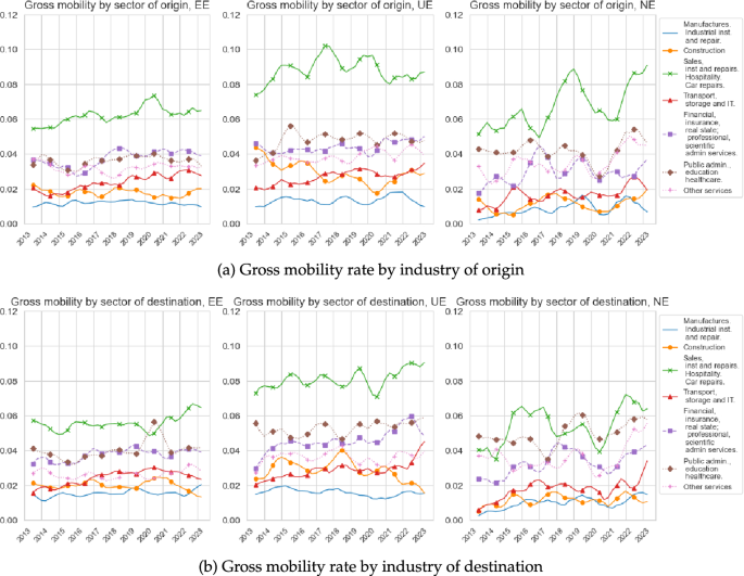
Source: Labour Force Survey
Gross industry mobility by origin and destination. The top panel depicts the gross mobility rate of workers by industry of origin, while the bottom panel depicts the gross mobility rate of workers by industry of destination. Each of the three subfigures in each panel considers different type of transitions. The left subfigures depict the gross mobility among EE movers, the centre subfigures depict the gross mobility among EUE movers, and the right subfigures depict the gross mobility among EIE movers.
3.2 Key aggregate time series
Figure 1 shows the time series of gross mobility by origin and destination industry using the seven industries in the 1-digit classification for which we have vacancy data. Total gross mobility across industries averaged about 25% during the period of observation with a generalised positive trend since 2013, with the exception of some industries during the Covid-19 period. These figures show that we can roughly divide the degree of churning across industries into three groups. The first group consists of only “Sales, Hospitality and Repairs”, which exhibits the largest amount of churning across EE, UE and NE transitions, both receiving workers from other industries as well as sending workers to other industries. The second group, which exhibits similar levels of churning but below those of “Sales, Hospitality and Repairs”, consists of “Public Administration, Education and Healthcare”, “Financial, Insurance and Professional Services”, and “Other services”, where the latter sector mainly consists of “employers of domestic personnel” and “other personal service activities”.Footnote8 The last group exhibits a slightly lower amount of mobility across all types of transitions, and consists of “Transport, Storage, IT”, “Construction” and “Manufacturing”.
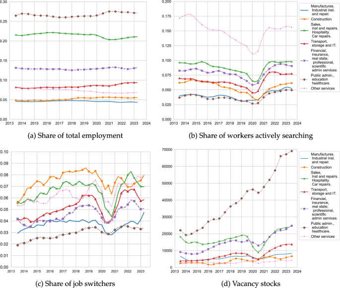
Source: Spanish Labour Force Survey and Labour Cost Survey
Employment, search activity, EE transitions and vacancies. Panel a gives the quarterly proportion of employed workers by industry. Panel b gives the proportion of employed workers who declared actively looking for jobs by the industry in which these workers were employed at the time of each survey wave. Panel c gives the quarterly employer-to-employer transition rates by industry of origin. Panel d gives the quarterly time series of vacancy stocks by industries.
Figure 2a shows the share of workers employed, , in each of these seven industries. The importance of “Public Administration, Education and Healthcare” as the largest employing sector is evident from its relative size, followed by “Sales, Hospitality and Repairs”. For the analysis that follows, we highlight that “Other Services” has seen its employment share decrease since 2013, while “Construction” has seen a mild increase in its employment share such that by 2022 and 2023 the difference in these sectors’ shares has halved. In Appendix A, we decompose the industry-specific employment shares by demographic characteristics, showing that “Public Administration, Education and Healthcare” and “Other Services” are women-dominated sectors, where there is about twice as many employed women as men; whilst “Manufacturing” and “Construction” exhibit the opposite pattern. We also show that most of the workers employed across these industries have at most a high school degree, with the exception of “Public Administration, Education and Healthcare” that exhibits a much higher proportion of college graduates.
Figure 2b shows the quarterly time series of by each s. The condition requires for each s and at each t that the total search intensity of employed workers in such an industry equals the value of . Weighting employed workers by the proportion of search channels they were using when actively searching for jobs gives very similar values. This occurs as we do not observe too much variation in available search channels across workers.Footnote9 It is evident from the figure that the strongest search activity among the employed arises from “Other Services”. The remaining set of industries exhibit a much more similar share of employed workers actively searching for jobs. Note that even though “Other Services” and “Construction” show similar employment stocks, the proportion of workers employed in “Construction” who are actively searching for a job is about three times lower than that of “Other Services”. Appendix A shows that the main reason for this difference is that the share of women employed in “Other Services” and actively searching is twice as large as that of men, while these shares are about the same for “Construction” and the other industries. Further, the within industries shares of active searchers are also similar across education and nationality groups, leaving the gender dimension as the main reason behind the observed high search activity of workers employed in “Other Services”.Footnote10
Figure 2c depicts for each industry of origin s as the share of those employed workers who made an employer-to-employer transition across two consecutive quarters. Here we aggregate workers who found new employers either in their same industry s or in another industry . A striking feature of this figure is the similarity between the employer switching rates of “Construction” and “Other Services”, particularly in the aftermath of the Covid-19 recession. This is striking given that we find a much higher proportion of employed workers actively searching in “Other Services” than in “Construction”. In Appendix A, we show that although the employer-to-employer transition rates starting from “Other Services” do not meaningfully differ by gender, we do observe an overall higher employer-to-employer transition rate among male construction workers than female construction workers.
Figure 2d shows the quarterly time series of the vacancy stocks by industry. As widely documented in the literature, vacancies exhibit a procyclical behaviour. Once again we can observe the importance of “Public Administration, Education and Healthcare” for the Spanish labour market. This sector exhibits the fastest rate and the largest amount of vacancies posted since 2013.Footnote11 This sector is followed by “Sales, Hospitality and Repairs” and “Financial, Insurance and Professional Services”, whilst “Transport, Storage, IT”, “Construction”, “Manufacturing” and “Other Services” exhibit the lowest and very similar amounts of vacancies posted.Footnote12
In conjunction with the unemployment and inactivity stocks by industry, the above figures present all the data inputs we require to estimate our model. In what follows we will smooth model generated data using a centred 5Q moving average and compare this to the data series using a similar smoothing procedure. This slightly de-phases model and data time series with episodes like the pandemic and the Spanish 2022 labour reforms. We highlight that given the similarities in “Construction” and “Other Services” employment shares, reallocation rates and vacancies stocks, Fig. 2 implies that the key differential feature between these sectors arises from the search activity of its employed workers, particularly from the female workforce. We return to this feature below.
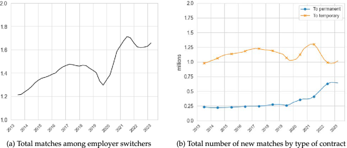
Source: Spanish Labour Force Survey
Total Numbers of Matches in Spain, 2013–2023. The left panel depicts the quarterly time series of total number of matches formed by workers that made an EE, UE or IE transition as measured by the Spanish LFS. The right panel decomposes these matches by the type of contracts workers declared they have been employed in.
3.3 Aggregate matching function dynamics
Figure 3 shows the quarterly time series of the number of matches, , observed among workers who made an EE, UE or IE transition between 2013 and 2023. The left panel shows that the number of matches among employer switchers increased during the pre-pandemic period, albeit at a decreasing rate; and after falling during the pandemic years, it started increasing at a fast rate only to dip and then continue its recovery towards the end of the period. The right panel decomposes these matches by whether they were formed under a permanent or temporary contract (information obtained from the LFS). We observe that the majority of new matches formed by employer switchers are under temporary contracts, highlighting the duality of the Spanish labour market. For now, we will focus on total matches and differentiate between types of contracts below.
Although both our sectoral model and the canonical DMP model replicate the time series of , each model implies a very different underlying picture. Figure 4 depicts the time series of the components of the matching function in the DMP model and compares them with the corresponding ones obtained from our sectoral model. Recall that our model does not exhibit an aggregate matching function, but a set of sector-specific matching functions all sharing a common elasticity , estimated to be 0.65. For comparability, we aggregate our estimated search intensities into and use the common time series component of as our measure of aggregate matching efficiency. For the DMP model, we estimate an aggregate Cobb-Douglas matching function, using as inputs the observed time series of and to obtain estimates of and .Footnote13
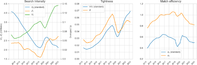
Source for and : Spanish Labour Force Survey and Labour Cost Survey
Series of matching function components. The left panel depicts the time series of the estimate aggregate value of workers’ search intensity, , and the observed unemployment and vacancy rates. The middle panel depicts the values of the two measures of labour market tightness (implied by sectoral model) and (implied by the standard DMP model). The right panel gives the estimated time series of the matching efficiency parameters implied by the sectoral model and the DMP model.
Figure 4 suggests two main takeaways from this exercise. First, our model shows that after several years of decline, the pandemic appears to have generated a significant reversal in the trend of aggregate search intensity. The large and (mostly) continued increase in since the pandemic arises against a backdrop of (mostly) growing vacancy creation and declining unemployment rate. Since vacancies grew faster than the decline in the unemployment rate, the canonical DMP model implies that by 2023 the Spanish economy was suffering the highest level of labour shortages in a decade. In contrast, when taking into account the estimated search intensity across industries, we observed that aggregate labour market tightness peaked right before the pandemic and by 2023 it was about 1.1 percentage points below this peak.
Second, the differential behaviour in labour market tightness implies a much stronger fall in matching efficiency since the pandemic in the sectoral model relative to the DMP model. Our estimates shows that matching efficiency in 2023 was close to a 10-year low, similar to the one estimated for 2014.Footnote14 Figure 5 further explores this last implication by depicting the estimated behaviour of the aggregate and sectoral job finding rates (per unit of search intensity) in relation to the corresponding values of matching efficiency.
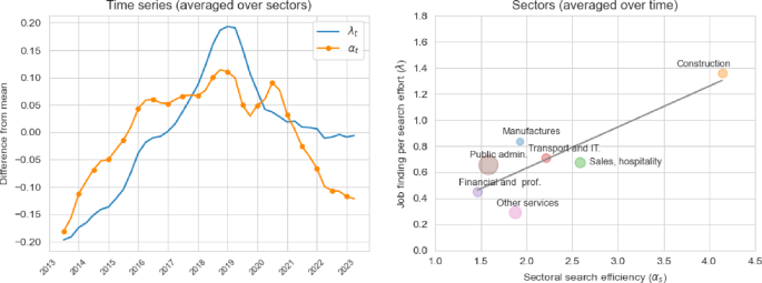
Estimated job finding rates and matching efficiencies. The left panel depicts the time series of the aggregate values of and , where the former is the time-varying component of and the latter is obtained by an employment-weighted average of at each t. The right panel shows a scatter plot of the relation between the averaged values of for each s and the corresponding fixed effect
Given our parameterisation, the sector-specific job finding rate is given by . The left panel of Fig. 5 shows the time series of and , where the latter is obtained by an employment-weighted average of at each t. We find that the job finding rate also exhibits a similar humped-shape behaviour as does , both peaking around 2019. The fall in aggregate matching efficiency and of labour market tightness have contributed to the drastic fall in immediately after its peak. However, the key reason way continued to fall despite an (overall) increase in labour market tightness after the pandemic was due to the drop in . That is, in the aftermath of the pandemic the average Spanish worker found it much harder to find employment because of the drastic drop in matching efficiency.
The main reason why we observe a decreasing value of and after the 2019 has to do with how our model squares the dynamics of workers EE transitions across sectors together with the rise of search effort. At an aggregate level, Fig. 2 implies that the average search effort of all employed workers more than double during the 2019 to 2023 period, and by 2023 it achieved its highest level in a decade. However, the dynamics of the EE transitions rates was more subdued. Although decreasing at the beginning of the Covid-19 pandemic and the rising in its aftermath, the values of did not increase above their pre-pandemic levels for the vast majority of industries. The model resolves this tension by estimating a decreasing and . That is, we observe that workers were exerting more search effort, but this did not fully translate into a proportionally higher reallocation rate. Thus, through the lenses of our model, the job finding rate per unit of search efficiency must have been falling. Given the overall rising in labour market tightness after 2020 depicted in Fig. 4, the reason behind the decrease in must be a falling .
Behind these aggregate patterns, the right panel of Fig. 5 shows that there is a large amount of heterogeneity across industries. This figure presents a scatter plot of the relationship between the time-averaged values of and , where the employment size of each industry is depicted through the size of the circle associated with such an industry. The (overlaid) line shows a clear positive relationship between these two variables, where “Construction” presents the largest matching efficiency and job finding rate, whilst “Other Services” present the lowest job finding rate and the third lowest matching efficiency. The main reason behind the large differences in the values of and between these two sectors is the large difference in their employed workers search activity as documented earlier. With similar levels of EE transitions rates and vacancy stocks but a large difference in , the model estimates lower values of and for “Other Services” but much higher values for “Construction”.
Given that the total number of matches is given by , where
and since continuously decreased since its peak, our model implies that the behaviour of the number of matches during the aftermath of the pandemic, as depicted in Fig. 3, has been mostly determined by the increase in search intensity (as shown in Fig. 4).
3.4 Search intensity across employment status and contract types
To investigate the behaviour of in more detail, Fig. 6 depicts the time series of total search intensity conditional on employment status, where , and denote the total search intensity of employed, unemployed and inactive workers, respectively. The figure also depicts the behaviour of aggregate search intensity units , and and the stocks , and . Given that unemployed workers have an average search intensity that is about 3 to 4 times larger than that of employed workers and 6 to 8 times larger than that of inactive workers , Fig. 6 presents deviations from each time series’ long-run trend to better visualise their properties and ease comparability across these labour force states.
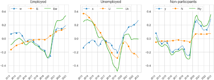
Search intensity by employment status—deviations from long-run average. The left panel depicts the time series of total search intensity, , and decomposes into search intensity units, , and stocks, . The middle and right panels depict the same time series for the unemployed and inactive. We present deviations from each of these series long-run trends to ease comparability
Across employment status, we observe the same pattern we documented for in Fig. 4. To different degrees, there has been a decrease in , and until the start of the pandemic, a strong increase immediately after the pandemic and a decline and a rebound by the end of the period. For employed and inactive workers the decrease in the pre-pandemic period was mainly driven by and , while for the unemployed the decrease was mainly driven by the falling numbers of unemployed workers. In the aftermath of the pandemic we observe a steep increase in all , and , with a much smaller dip for and than in towards the end of the period.
These graphs make it clear that the post-pandemic behaviour of , and strongly shaped that of , and and hence of . Hence, total matches among employer switchers increased in the aftermath of the pandemic as search intensities across all employment status categories increased more than the decrease in the job finding rates per unit of search intensity.
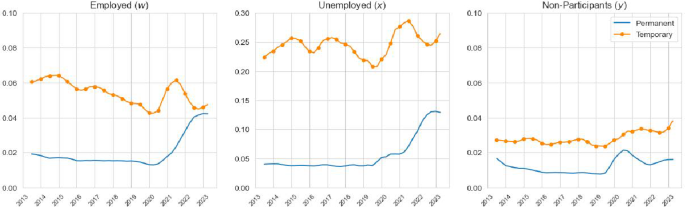
Search intensity towards permanent/temporary contracts. The left panel depicts the time series of search intensity units among employed workers, , that can be attributed to moves towards permanent or towards temporary contracts. The middle and right panels depict the same time series for the unemployed and inactive. We present the estimated search intensities in levels
Figure 7 further decomposes , and by whether the worker ended up employed in a permanent or temporary contract. Given that the vacancy survey does not provide information about whether a posted vacancies is associated with a permanent or temporary contracts, our decomposition is only possible under the assumption that workers who ended up employed in a permanent contract face the same as those workers who ended up in a temporary contract in the same sector. Although this is an undoubtedly a strong assumption in the context of Spain’s dual labour market, the decomposition shows some interesting results. In particular, we find that search intensity towards temporary contracts is higher than for permanent contracts, particularly for unemployed workers. Further, the rebound of search intensity since the pandemic occurred towards both temporary and permanent contracts. For the unemployed and inactive we observe a stronger overall increase (relative to the employed) in search intensity towards temporary contracts; whilst for the employed and unemployed we observe a stronger and sustained increase (relative to the inactive) in search intensity towards permanent contracts. These results suggest that the post-pandemic increase in search intensity was not driven by one part of the Spanish dual labour market, but it occurred in both.
3.5 Search intensities across industries
A key feature of our framework is that it allows us to evaluate workers’ search intensities across industries. The top row of Fig. 8 shows the search intensities of employed, unemployed and inactive workers that originates from the seven industries we use. We observe that the strongest search intensity across the different employment status originates from the “Other Services”. Since we use the observed search effort of employed workers by industry of origin in our estimation, it is not surprising that the resulting time series for w in the left panel follows closely the empirical series documented in Fig. 2, where the search intensity originating from “Construction” remains three times lower than that of “Other Services”. Although we do not use information on the search effort of unemployed or inactive, we also observe that among the non-employed a large difference between the search intensity originating from “Other Services” and “Construction”.
The bottom row of Fig. 8 instead shows the search intensities of employed, unemployed and inactive workers towards these seven industries. We observe that now the search intensities towards “Sales, Hospitality and Repairs” is the strongest one for the employed and unemployed workers, followed by “Other Services”; while for inactive workers the strong search intensity towards “Sales, Hospitality and Repairs” is shared with “Other Services”. Note that even in this case the difference between the search intensities towards “Other Services” and “Construction” is even larger, particularly for the unemployed and inactive. These differences in search intensities underpin the resulting differences in these sectors matching efficiencies parameters as discussed earlier.
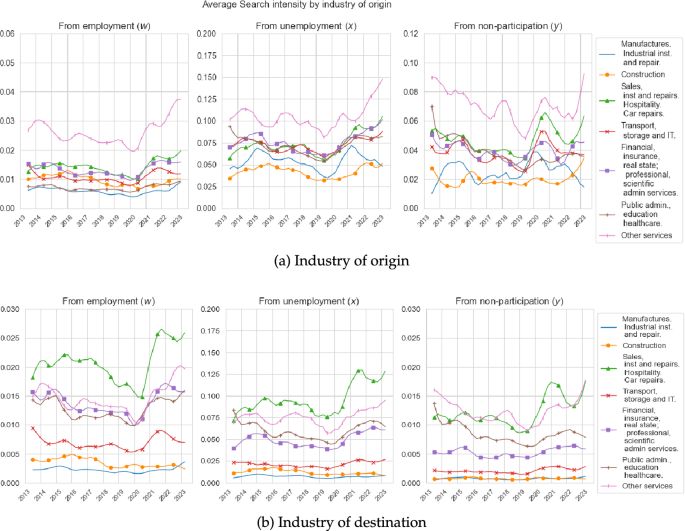
Search intensity w, x and y by industry. The top row depicts the estimated time series of search intensity units originating from each individual industry among the employed (left), unemployed (middle) and the inactive (right). The bottom row depicts the estimated time series of search intensity units directed towards each individual industry among the employed (left), unemployed (middle) and the inactive (right). We present the estimated search intensities in levels
Although not shown here we also further decompose workers’ search intensities towards various industries by type of contract. Across employment status and contract types, we observe that the industry ranking described above remains. In line with Fig. 7, we find that for most of the period the search intensity towards permanent contracts in any given industry is lower than the search intensity towards temporary contracts in the same industry.Footnote15 In Appendix C, we further investigate our search intensity estimates by showing that the proportion of search intensities that is directed towards workers own industries is larger and the proportion that is directed towards other industries, consistent with the gross mobility rates documented in Fig. 1. In this appendix, we also provide a decomposition of the aggregate gross and net mobility rates and show that variation in search intensities across sectors and time is the main driving force behind the cyclical properties of gross and net mobility.
The main takeaway from these results is that since “Sales, Hospitality and Repairs”, “Public Administration”, “Financial, Insurance and Professional Services” and “Other Services”, exhibit the lowest job finding rates and matching efficiencies (as documented in Fig. 5), the main reason why we observe large gross flows towards these industries is because workers across employment status and type of contracts exhibit relatively large search intensities from and towards these industries. This observation is verified in Sect. 4.2, Fig. 11, where we investigate the estimated search intensity directed across different industries relative to the optimal one implied by the Match Maximising Allocation.
4 Labour shortages revisited
Taken together, the results in the previous sections suggest that search intensity is the main driver of worker reallocation across industries in the Spanish labour market. If worker reallocation is key to understand flows across industries, then why labour shortages remain high, although not as high as during the pandemic? We now turn to tackle this question.
4.1 Post-pandemic labour shortages
An advantage of our framework is that it delivers estimates of market tightness (or shortages) by industry, such that
We can then use the change in to evaluate whether labour shortages arose due to an increase in vacancies in a given industry or a decrease in search intensity towards that industry. In particular, we can use , such that implies sector s is receiving more search intensity from the same sector and/or other sectors, while implies a reduction in labour shortages in sector s.
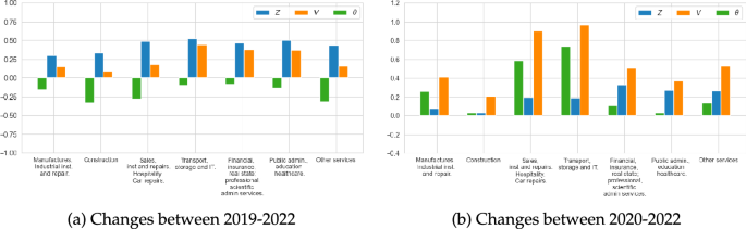
Decomposing labour shortages by industry. The left panel depicts changes in log labour market tightness, log search intensity and log vacancies for the period 2019–2022. The right panel depicts these changes for the period 2020–2022
Figure 9 shows the decomposition of the change in industry labour market tightness in terms of changes in search intensity and in vacancies. We present this decomposition for two overlapping periods: 2019–2022 and 2020–2022 in order to compare the extend of labour shortages observed immediately before and after the pandemic. Between 2019–2022, we observe that such that aggregate labour shortages fell due to higher search intensity across for all industries. When comparing 2022 against 2020, however, we observed an increase in labour shortages, and this was due to a stronger increase in vacancies relative to search intensity. This is because the increase in search intensity occurred before the post-pandemic rebound in the growth of vacancies. Perhaps it is the comparison with 2020 that explains why there has been so much interest in tackling labour shortages in economies like the Spanish ones. However, under both scenarios labour shortages remain high.
4.2 Match maximising allocation
The above analysis suggests that workers might not be searching hard enough in those industries which experienced the largest increases in vacancies or offer better job finding prospects and hence one could think of rearranging workers’ search intensities to maximise the number of matches. That is, how well are search intensities allocated across industries, conditional on where firms are posting jobs and industry-specific ? We answer this question by deriving the match maximising allocation (MMA). The MMA gives the distribution of search intensities that would maximise the total number of new matches in a given period t, holding aggregate search intensity and the distribution of fixed in such a time period. Namely,
subject to .
Note that our approach is slightly different from that of Şahin et al. (2014), who consider socially optimal distribution (conditional on model), not the match maximising distribution. However, as in their paper we obtain that the solution to our MMA is given by equalising the marginal increase in job finding rates per unit of search intensities across industries,
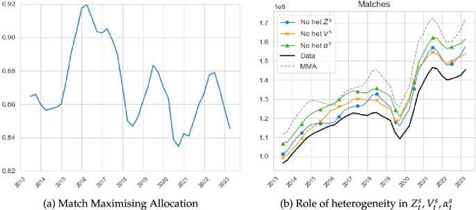
Match maximising allocation and total matches. The left panel depicts the ratio between total matches and the matches implied by the MMA. The right panel depicts total matches, the matches implied by the MMA as well as counterfactual eliminating heterogeneity in , and
The left panel of Fig. 10 depicts the ratio between total matches and the total number of matches implied by the match maximising allocation, . Notice that if this ratio were to be equal to one, the labour market would be allocating search intensity in accordance with the MMA rule. The lower is this ratio, however, the further is the economy from the optimal allocation. The figure shows that since 2016 the Spanish labour market has been trending further away from the MMA allocation, with dramatic drops in 2018, during the Covid-19 pandemic and after the labour reforms of 2022. By the end of the period of observation, the Spanish labour market was allocating quite poorly search intensities across industries.
The right panel of Fig. 10 shows the series of total matches (as in Fig. 3) and the one implied by the MMA. Their ratio is what has been plotted in the left panel of the figure. In addition, we show the result of three counterfactual exercises. Since to achieve the MMA we need to equalise the marginal job finding rates across sectors, we can use this condition to evaluate the effect of separately equalising search intensities, matching efficiencies or vacancies across industries, the three components that create dispersion in . We perform these counterfactuals by only equalising each of the three components at a time, setting each (independently) to their average levels for each t, while respecting the heterogeneity in the other two. Figure 10 shows that by equalising either or total matches are increased by roughly the same amount, halfway between the and series. Equalising has the largest impact, increasing total matches much closer to the series. This result implies that in the Spanish labour market not enough search intensity is allocated to sectors with high .
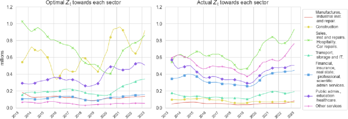
MMA and estimated by industry. The left panel depicts the aggregate search intensities directed towards different sectors that are obtained from the MMA. The right panel depicts the aggregate search intensities directed towards different sectors that are obtained from our estimation
Figure 11 makes clear this implication. The left panel shows the values of for each industry implied by the MMA rule, while the right panel shows the values of implied by our original estimation. Comparing the two panels shows that to maximise the number of matches in the post-pandemic period, search intensities towards the “Construction” sector should be about 8 times higher than what is estimated to be, while search intensity towards “Other Services” and “Financial, Insurance and Professional Services” should be about 8 and 2 times lower. The search intensities towards the reminder industries are about right relative to the ones implied by the MMA.
The reason why our model predicts that a reallocation of search intensity towards the “Construction” sector and a reduction of search intensity towards “Other Services”, rests on these industries matching efficiency differentials. As shown in Fig. 5 and discussed in previous sections, “Construction” exhibits the highest and , while “Other Services” exhibits the lowest and the third lowest . Given that over time both have roughly had the same number of vacancies posted (see Fig. 2c) and similar employment sizes and reallocation rates, it is intuitive that one should increase search intensities towards the industry exhibiting the highest job finding probability per unit of search intensity to achieve the MMA.
Here it is important to note that the MMA is the allocation that maximises the fluidity of the labour market. It is not the allocation that minimises unemployment or non-employment, as we will need to take into account the flows out of employment to stablish this. Consider an economy with two sectors, one with high and high job destruction rate and another with lower and a lower job destruction. The MMA would recommend to send more workers to the sector with high , but this will result in higher stock of unemployment at any point in time. That is, more unemployed workers with shorter unemployment spells. This example points to a policy trade-off between a more fluid but volatile economy and a more stable one with higher unemployment. However, analysing this trade-off is beyond the scope of our paper. The MMA points out that if we want to make the hiring market more efficient, we should reallocate workers towards sectors where it is easy to find jobs, but it does not say anything about how long these jobs last.
Through this lens, “Construction” is a sector where it is very easy to find jobs with very minimal search effort. In contrast, it takes comparatively more time to find jobs in “Other Services”, a category that encompasses a variety of jobs: hairdressers, beauticians, gym instructors, entertainment industry and politics, to name the most salient. Therefore, reallocating searchers from “Other Services” to “Construction” can create more matches because the comparatively low skill requirements and homogeneity of the jobs in the “Construction” sector. Fixing the curvature of the matching function, this difference is absorbed in our model by .
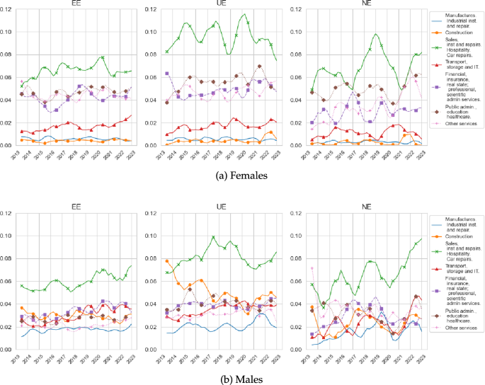
Source: Labour Force Survey
Gross industry mobility by destination. The top panel depicts the gross mobility rate of workers by industry of destination, disaggregated by gender. Each of the three subfigures in each panel considers different type of transitions. The left subfigures depict the gross mobility among EE movers, the centre subfigures depict the gross mobility among EUE movers, and the right subfigures depict the gross mobility among EIE movers.
Another interpretation of our results arises when we observe employment flows separately by gender: “Construction” is a very male-dominated sector, while “Other Services” is more balanced. Figure 12 shows that women’s destination industries are concentrated in the core 4 service sectors, while for men they have more diversified flows. Notice that “Construction” is a prominent destination for men, while negligible fore women. Because the MMA allocation is achieved when we equate job finding rates across all sectors, having some workers never search in “Construction” might be generating congestion in the services sectors.
5 Conclusion
In this paper we have used a sectoral matching framework to investigate the role of workers’ search intensities across industries in determining the evolution of the number of new matches among employer switchers in the Spanish labour market. Our framework allows us to disentangle the different contributions of firms’ vacancy postings, workers search intensities and matching efficiency at a sectoral level. Firms’ vacancy postings capture labour demand effects in match formation, while search intensity captures labour supply effects. Matching efficiency captures the effectiveness of match formation due to sector-specific practices, technology, and firm recruitment policies, among other dimensions and it is assumed to be independent from workers’ search intensity.
We estimate our framework on readily available LFS and Vacancy survey data from 2013 to 2023 and show that aggregate search intensity has been steeply increasing since the pandemic, marking a reversal from the previous downward trend. This increase was propelled by an increase in search intensity across employment status, towards permanent contract among the employed and unemployed and towards temporary contracts among the non-employed, and directed mostly towards “Other Service” and “Hospitality/Sales”, which are relative low matching efficiency and low job finding rate industries. Importantly, given that the aggregate matching efficiency and job finding rate decreased since the pandemic, the rise in total matches observed since the pandemic has been due to the increase in search intensity. This result presents a different perspective relative to the standard DMP model about the state of labour shortages in Spain. While the DMP framework would imply that by 2023 labour shortages were at a 10-year high, we find that when taking into account sectoral reallocation shortages are lower in 2023 than immediately before the pandemic, but do remain high.
To investigate the persistence of labour shortages, we use our framework to evaluate whether search intensities are allocated across industries in a way that maximises the total number of new matches, given the observe distribution of vacancies and matching efficiencies across industries. We find that the allocation of search intensity has been trending further away from the optimal allocation such that by 2023 this allocation is closer to the lowest point observed in the last decade. This misallocation is primarily due to the differences in matching efficiencies across industries. We find that to maximise the number of new matches search intensity should be much higher towards high matching efficiency industries like “Construction”, while search intensity towards low matching efficiency industries like “Other services” should be much lower relative to the estimated search intensities. Taken together these results imply that in Spain labour mobility does not seems to be driven by firms’ vacancies postings (labour demand) but by workers’ search intensity (labour supply) suggesting a larger role for matching frictions, as opposed to “just create more jobs”, in the creation of new matches and the further reduction of labour shortages.
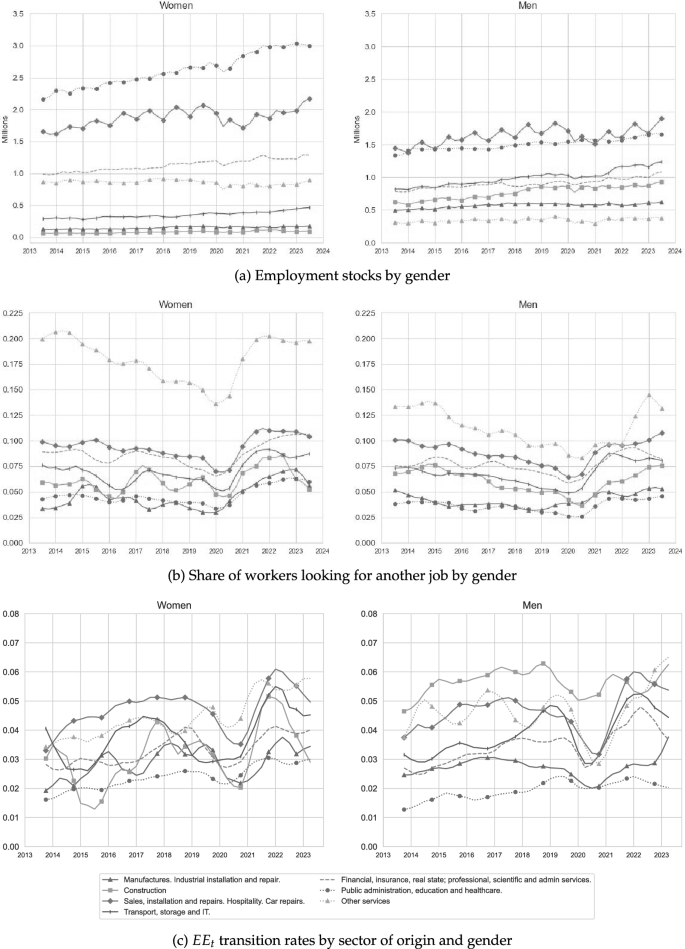
Employment, search intensity and employment flows, by gender
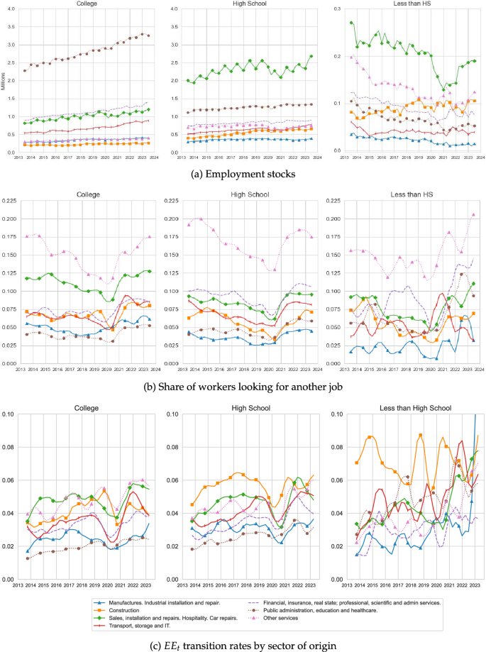
Employment, search intensity and employment flows, by education
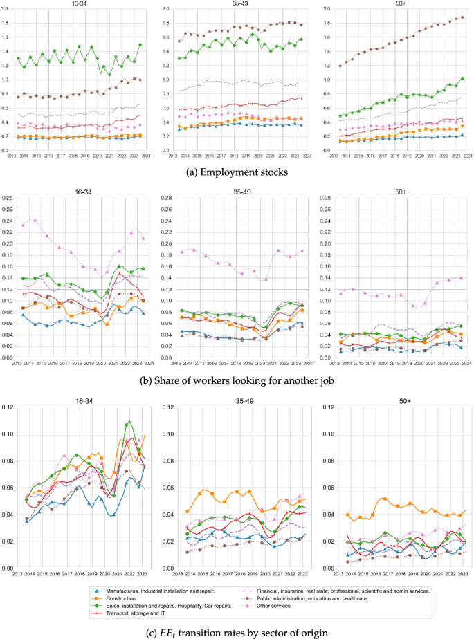
Employment, search intensity and employment flows, by age
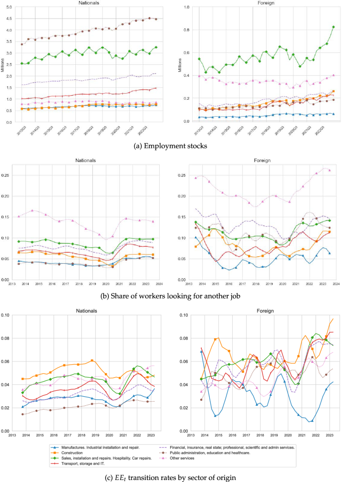
Employment, search intensity and employment flows, by nationality
A potential concern is that our analysis has assumed that all industry-specific matching functions share a common elasticity . In Appendix D, we estimate an alternative version of the model allowing for sector-specific elasticities . The main message from this exercise is that search intensity should be directed even more strongly towards “Construction” rather than “Other Services”, as “Construction” not only retains its high matching efficiency but now vacancies exhibit a more important role in match formation, with an estimated elasticity .
Data availability
The data outlined in our article are obtained from the “Instituto Nacional de Estadistica” (INE) of Spain. The data on vacancies come from the “Encuesta Trimestral de Costes Laborales” (ETCL), Resultados nacionales (desde el trimestre 1/2008), Vacantes. This is public information compiled by the INE. The data on labour market flows comes from the “Encuesta de Poblacion Activa” (EPA). We requested the confidential version on labour market flows that includes a link variable. This needs to be requested to the INE and approved for scientific use. You can apply for the data through their web portal. We only provide aggregate results for the analysis, in compliance with the confidentiality agreement with the INE.
Notes
-
This result is not at odds with our finding that persistent labour shortages arise as workers are not searching more intensively in high job finding rates industries. The latter relates to the distribution of matching efficiencies and job finding rates, while the former to their evolution of time.
-
We allow for search intensity from employed and inactive workers, and for search intensity to be directed to other industries. These extensions are pursued separately in Şahin et al. (2014), using different approaches than the one in this paper. Şahin et al. (2014) find, in the US, that the bulk of unemployed workers keep searching in their previous sector.
-
As in Garibaldi and Wasmer (2005) and Elsby et al. (2015), we will consider inactivity as another labour market state, in conjunction with employment and unemployment, in which individuals search with (potentially) lower intensity. This implies that these workers have the possibility of becoming employment instead of not participating at all in the labour market. Considering inactivity as separate labour market state where workers have the possibility of encountering job opportunities is important to explain sectoral labour flows as we observe many individuals who declared being inactive in a given period but found employed in the subsequent period. In previous studies, these workers have been labelled as marginally attached and are shown to behave in many dimensions as regular unemployed workers (Jones and Riddell 1999).
-
For example, if a worker employed in a sector s declares active job search at time t, we record this by using an indicator function that takes the value of one if there is active job search and zero otherwise. We then multiply an affirmative answer by the proportion of search channels he/she declared using at time t. Given the total amount of search channels specified in the survey from which the worker can choose from, , the proportion would be given by , where denotes the number of channels actually used at time t. is then obtained as the sum across all employed workers in sector s, where those who are not actively searching will have a zero attached to their observation and those who are actively searching would have their corresponding attached to their observation. In the Spanish LFS we observe across our window of observation. See Appendix B for the description of these search channels as well as their long-run average usage and how usage changes over time.
-
Shimer (2004) uses this formula but for unemployed workers. In that case, he takes all unemployed as actively searching and hence the numerator is equal to the sum of the proportion of search channels used by each unemployed worker, whilst the denominator is equal to the number of unemployed workers. Mukoyama et al. (2018) extends Shimer (2004) by re-weighting the proportion of search channels each unemployed worker uses by the minutes they declare using them in the American Time Use Survey. Although we are not able to use Mukoyama et al. (2018) approach to construct due to the lack of data, our framework does allow it as the scale through which is measure in the data works as a normalisation. This is because Eqs. (3), (4), (5) and (6) as well as and imply that any proportional change in the level will proportionally re-scale our estimated values of , , and ultimately . We also chose not to focus on the unemployed (or inactive) to measure search effort as in our application to the Spanish LFS we do not observe the industry of origin s for those individuals who have been unemployed (or inactive) for more than a year, biasing our measure towards those with “shorter” unemployment spells. By using employed workers we avoid this problem.
-
For a simple example suppose that workers only made employer-to-employer transitions within their own sector, so that for all , and . The identification from (6) then simplifies to giving . In this case, the job finding rate per unit of search intensity is identified as the employer-to-employer rate of workers in that sector divided by the reported search effort of workers in the same sector. The case with cross-sector flows is similar, and just weights the reported search efforts according to the pattern of cross-sector employer-to-employer rates.
-
Formally, we create an “”th industry for stocks and flows with missing data. Since we drop flows where the receiving job has missing data, we thus have sending industries and S receiving industries. This does not change the logic of the model or estimation at all, and simply allows us to back out and analyse the search intensity of the workers with missing industry data in parallel with the other workers.
-
These two sub categories account for about 60% of employment in the “Other Service” industry during the period of observation. “Sports activities” and “activities of other memberships organisations” account for another 20%. The remaining 20% is accounted by employment in “activities of extraterritorial organisations and bodies”, “repair of personal and household goods”, “repair of computers and communication equipment”, “activities of trade unions”, “activities of business, employers and professional membership organisations”, “amusement and recreation activities”, “gambling and betting activities”, “libraries, archives museums and other cultural activities”, and “creative, arts and entertainment activities”.
-
The average number of search channels used is 3.7, where the vast majority of employed workers actively searching for a job declared that they have “have reached out to family and friends”,“have reached out to entrepreneurs or HR teams”, “checked jobs ads on any media” and“have posted an ad in any media”. They also report to “have contacted private employment services” and “have contacted a public employment office”. See Appendix B for further details.
-
Aggregating across the quarterly time series depicted in Fig. 2b generates . This measure of aggregate search effort exhibits the same procyclical behaviour as the individual time series, with a steep rebound after the Covid-19 recession, inline with the conclusions of Shimer (2004) and Mukoyama et al. (2018) based on unemployed workers. Note also that our identification condition requires that . Hence the model time series of is equal to the empirical measure of obtained from the LFS. Further, since the measures of are identified from the transition rates , we use the condition as a restriction on these to identify the matching efficiency parameters, .
-
A potential concern is that the steep rise of “Public Administration, Education and Healthcare” vacancies might be driving most of our results, particularly as one reason for this increase is due to the delay in “concursos”. However, since we estimate our model period by period, what matters for our estimation is the relative level of vacancies (as well as the relative level of other stocks) and not necessarily the speed at which they grow.
-
Although there is size variation across these industries, the differences are not that large compared with the difference between them and “Public Administration, Education and Healthcare”. We once again emphasise that the data quality of the vacancy series provided by the ETCL has some selection issues, as outlined above. Our analysis could then be affected by biases in the data and hence our results should be interpreted keeping this in mind.
-
The estimated value of the in the DMP model is 0.71, which is slightly higher than in our sectoral model suggesting that considering worker sectoral flows reduces the role of vacancies in the probability of matching. These estimates are based on OLS regression. Borowczyk-Martins et al. (2013), however, show that these estimates are upward bias due to the endogenous search behaviour of firms and workers in the DMP model. We considered the IV correction method proposed by Borowczyk-Martins et al. (2013) and found that our conclusions are not meaningfully affected.
-
Note that although one typically finds estimated matching efficiency to be procyclical in relation to the aggregate unemployment rate, the Covid-19 pandemic changed this dynamic. In both the DMP and the sectoral model behaved in tandem with unemployment, with the strongest fall in implied by our model.
-
The main exception is the search intensity employed workers exhibit towards permanent contract in the “Sales, Hospitality and Repairs” industry, which is higher than for temporary contracts by the end of the period.
References
-
Borowczyk-Martins D, Jolivet G, Postel-Vinay F (2013) Accounting for endogeneity in matching function estimation. Rev Econ Dyn 16:440–451
-
Busch C, Galvez-Iniesta I, Gonzalez-Aguado E, Visschers L (2024) Dual labor markets, unemployment and career mobility. Working papers, Department of Economics, Universidad Carlos III
-
Carrillo-Tudela C, Visschers L (2023) Unemployment and endogenous reallocation over the business cycle. Econometrica 91:1119–1153
-
Carrillo-Tudela C, Hobijn B, She P, Visschers L (2016) The extent and cyclicality of career changes: evidence for the U.K. Eur Econ Rev 84:18–41
-
Carrillo-Tudela C, Clymo A, Comunello C, Jäckle A, Visschers L, Zentler-Munro D (2023) Search and reallocation in the COVID-19 pandemic: evidence from the UK. Labour Econ 81:102328
-
Carrillo-Tudela C, Clymo A, Comunello C, La Fuente C, Visschers L, Zentler-Munro D (2024) Sector mobility and labour shortages: a cross-country analysis. Working paper, Department of Economics, University of Essex
-
Cortes GM, Jaimovich N, Nekarda CJ, Siu HE (2020) The dynamics of disappearing routine jobs: a flows approach. Labour Econ 65:101823
-
Costa Dias M, Johnson-Watts E, Joyce R, Postel-Vinay F, Spittal P, Xu X (2021) Worker mobility and labour market opportunities. IFS working paper, 21
-
Diaz A, Dolado J, Janez A, Wellschmied (2024) Labor reallocation effects of furlough schemes: evidence from two recessions in Spain. Eur Econ Rev (forthcoming)
-
Elsby M, Hobjin B, Sahin A (2015) On the importance of the participation margin for labor market fluctuations. J Monet Econ 72:64–82
-
Faberman RJ, Mueller AI, Austin UT, Topa G (2021) Job search behavior among the employed and non-employed. Econometrica 70 (forthcoming)
-
Garibaldi P, Wasmer E (2005) Equilibrium search unemployment, endogenous participation, and labor market flows. J Eur Econ Assoc 3:851–882
-
Jones S, Riddell C (1999) The measurement of unemployment: an empirical approach. Econometrica 67:147–162
-
Kambourov G, Manovskii I (2008) Rising occupational and industry mobility in the United States: 1968–97. Int Econ Rev 49:41–79
-
Mukoyama T, Patterson C, Şahin A (2018) Job search behavior over the business cycle. Am Econ J Macroecon 10:190–215
-
OECD (2024) Employment outlook. OECD, Technical report
-
Patterson C, Şahin A, Topa G, Violante GL (2016) Working hard in the wrong place: a mismatch-based explanation to the UK productivity puzzle. Eur Econ Rev 84:42–56
-
Şahin A, Song J, Topa G, Violante GL (2014) Mismatch unemployment. Am Econ Rev 104:3529–3564
-
Shimer R (2004) Search intensity. Working paper, Department of Economics, University of Chicago
Acknowledgements
Funding from Fundación BBVA, an impact grant from the University of Edinburgh, and by grants CEX2021- 001181-M and ATR2023-145734 funded by MICIU/AEI /10.13039/501100011033 (Unidades de Excelencia Maria de Maeztu, and Programa ATRAE, Spanish Government) is gratefully acknowledged.
Ethics declarations
Conflict of interest
The authors declare that they have no relevant or material financial interests that relate to the research described in this paper.
Additional information
Publisher’s Note
Springer Nature remains neutral with regard to jurisdictional claims in published maps and institutional affiliations.
This paper was presented at the 3rd Conference of the Spanish Economy (Santander) organised by the Bank of Spain and CEMFI under the title “Spanish Labour Market Duality, Labour Mobility and Labour Shortages”. We thank Juanjo Dolado for his insightful discussion and conference participants for their helpful comments. We also thank two anonymous referees for their comments and suggestions. All errors are our own.
Appendices
A Employment shares, EE transitions and search effort
Our study treats all workers as homogeneous, but we know there are noticeable differences in observables. Figures 13, 14, 15 and 16 replicate Fig. 2 for four different demographic groups: gender, education, age groups and nationality. The main difference we find is in the gender dimension. Figure 13a shows that women are concentrated in services, while men are more evenly spread across industries. “Public Sector, Education and Health Care” and “Sales and Hospitality” are the two largest sectors for both. However, “Other Services” is markedly more prevalent for women than men. The opposite is true of “Construction”. Figure 13b shows that also women in “Other Services” search more intensely for other jobs, which, together with the large flows into this sector depicted in Fig. 13c, reflect high churning within this sector. It is noticeable that men are not searching comparatively intensively in “Construction”, yet this sector is very prominent destination as shown in Fig. 13c. Through the lenses of our model, the Match Maximising Allocation (MMA) may be picking up these differences, which are rationalised as the “Construction” sector having a very large efficiency of allocating (male) workers, as they do not search particularly hard yet exhibit large flows. Conversely, there are a lot of (female) workers searching for jobs in “Other Services”, achieving similar levels of mobility. So the MMA allocates women away from “Other Services” into more efficient sectors, like “Construction”, to correct for the imbalance. This could reflect that gender segregation in the labour market leads to inefficiencies, as women tend to be stuck in low productivity, low stability sectors.
These differences are more marked than for education, age and nationality categories. For education, Fig. 14 shows that the largest difference comes from college graduates being much more likely to work in the public sector. This makes sense in the Spanish context, where most of these jobs require college degrees and passing a series of written examinations. Workers with secondary degrees work more often in “Retail and Hospitality” but have relatively equal shares of “Other Services” and “Construction”. This is the same for the least educated worker group, so the imbalance between “Other Services” and “Construction” is not coming from education alone, as both sectors employ low-skilled workers. These observations coincide with non-Spanish nationals, as shown in Fig. 16, who are employed in easy-to-access industries that overlap with the lowest educated group.
Looking at Fig. 15 one finds that young workers search more intensely and switch jobs more often than older workers, as documented in the literature. The overall pattern of search effort in panel (b) is still preserved, with “Other Services” being clearly higher than others in all age groups. Note how for older workers “Construction” has a higher job-to-job transition rate than “Other services” despite the search effort in the latter being much higher. This reinforces the findings of the MMA. As a final note, panel (a) of Fig. 15 shows that the labour force is indeed ageing: the number of workers that are 50 years of age or older has increased in the past 10 years in all industries, but it is particularly notable in the public sector, where now there are more workers in this age bracket than in the 35 to 49 years bracket. The increase in young people since 2020 is an indication of the newly created civil service positions, which came with a delay.
B Search channels
In the LFS workers that declare active search are asked whether they use particular search channels. This information allows us to construct a measure of “search effort” as other authors have considered. These channels are listed in Table 1. One caveat is that the search channel questions were replaced in the 2021 reform of the LFS, which now offers only one variable with the number of channels employed—and crucially, it is not available in the linked, confidential version of the data we use. We therefore use the results from 2013 to 2021 and impute the 2021 results for the remaining years.
We find that employed workers use on average 3.74 channels to search, with some variation across industries, as depicted in Fig. 17. The coefficient of variation (standard deviation relative to the mean or CV) is 0.52. Unemployed workers in contrast use 4.37 channels with a CV of 0.44. Figures 18 and 19 show that the three most common channels are through family and friends, contacting prospective employers directly and checking for job adverts in the media. In addition, most unemployed workers have contacted the unemployment office. There are no noticeable differences by gender, as Fig. 20 shows—but it is worth noting that workers in “Other Services” and “Construction” present a similar composition of search channels as shown in Fig. 17.
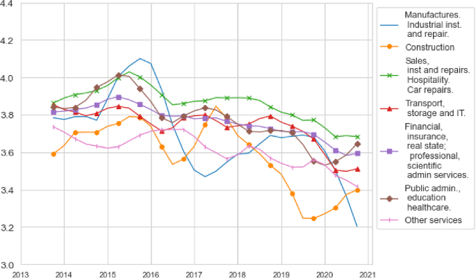
Average number of search channels, by current industry
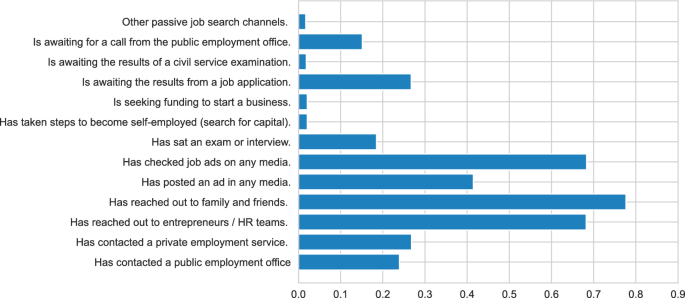
Average number of search channels, employed workers searching
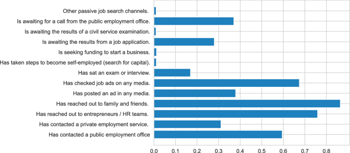
Average number of search channels, unemployed workers
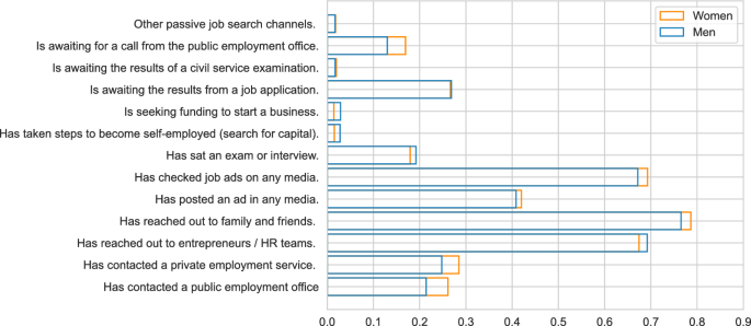
Average number of search channels, employed workers searching, by sex
C Worker reallocation across industries
In this section, we further develop Sect. 3.5 and investigate the implication of our estimates on gross and net mobility.
1.1 C.1 Search intensities within and across industries
Figure 21 shows that employed workers mainly direct their search towards their own industry, . In contrast, unemployed and inactive workers direct most of their search towards other industries, . Given that for the latter groups the difference between and is not too large, when aggregating across employment status we find that total search intensity towards workers own industries becomes larger than towards other industries. This is consistent with an aggregate level of gross mobility across industries below 50%, as documented in Sect. 3.2. Further, we observe that early on into the pandemic there was a stronger increase in , while in the aftermath there was a stronger increase in , resulting in the procyclicality of aggregate search intensity documented earlier.
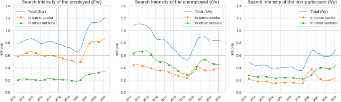
Search intensity within and across industries by employment status. The left panel depicts the time series of total search intensity among the employed, the search intensity directed towards their own industries and the search intensity directed towards other industries. The middle and right panels present the corresponding series for unemployed workers and the inactive. We present the estimated search intensities in levels
1.2 C.2 Decomposing gross and net mobility
The above results show that the level and evolution of and is consistent with the level and procyclicality of gross mobility across industries among employers switchers. However, gross mobility also depends on the to which these search intensities are directed. To understand the importance of relative to the other components of the job finding rate, and , we decompose the gross mobility rate. Noting that the aggregate gross mobility rate is given by
and that in our framework , and , substitution of these expressions results in
Rearranging and substituting using the definition of further gives
where denotes total search intensity towards sector from other industries. We use this last expression to recompute the series separately holding constant , or at their respective average levels at each t. That is, we evaluate the respective roles of sectoral heterogeneity across vacancies, search intensity and matching efficiency in determining gross mobility. The importance of each of these components is determined by the difference between the scale and cyclicality of the resulting series of and the one implied by the baseline model (and data).
The left panel of Fig. 22 shows the results from these counterfactuals. We observe a very small impact of in explaining changes in gross mobility. The series implied by imputing a common to all industries is nearly identical as the one observed in the data. Imputing a common instead generates a slight uplift in the gross mobility series suggesting heterogeneity in matching efficiencies across industries has mostly a level effect by not a cyclical one. Heterogeneity in search intensities, however, has a profound effect on the gross mobility series. By imputing a common across industries, the gross mobility rate not only changes its level, but also its cyclicality. Thus, it is clear that variation in search intensities across sectors is needed to explain the time series behaviour in the observed gross mobility rate.
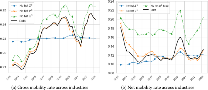
Decomposing gross and net mobility. The left panel depicts the time series of the gross mobility rate across industries together the counterfactual gross mobility series implied by holding fixed either , or . The right panel depicts the time series of the net mobility rate across industries together the counterfactual net mobility series implied by holding fixed either , or
The above exercise gives information about the drivers behind the total reallocation rate observed across industries, but does not allow us to investigate how the direction of such reallocation contributes to the change in the size of such industries. To evaluate the latter we consider the net mobility rate. This rate, as a fraction of gross flows, is given by:
where
and denote employment weights. Substituting , , and as above allow us to use the resulting expression to perform the same counterfactual exercise as done with the gross mobility rate.
The right panel of Fig. 22 shows the results of these set of counterfactuals. Note that in contrast to the gross mobility rate, net mobility is countercyclical, consistent with the evidence documented in Carrillo-Tudela and Visschers (2023) and Carrillo-Tudela et al. (2023). Nevertheless, we obtain similar conclusions as in the case of gross mobility. Even though variation of vacancies affects more net than gross mobility, appears as the less important force determining the level and cyclicality of . Heterogeneity in search intensities instead drastically change both the level and cyclicality, having a larger impact on the latter. Holding constant variation in matching efficiency creates a large level shift without meaningfully changing the cyclicality of the time series. In this case, the large level shift in reinforces the conclusion that workers are searching more intensely in industries that exhibit low and and that this reduces net mobility.
D Allowing for different curvatures
A related issue shows when we compare the results of our estimation when we assume a constant curvature of the matching function across sectors to when we let it vary by sector. In this case, we estimate by OLS the matching function
where we obtain by directly taking the implied from time-averaged data. Doing this allows us to compare the effects of the curvature or returns to scale () and matching efficiency (). Note that the residual absorbs the variation of match efficiency over time ().
Figure 23 compares the estimates we get from the regression where we let the parameter differ by industry (green dots in the left panels, green bars in the right panel) and our results in the main text, where we impose a common (blue dots on the left panel, blue line in the right panel). All estimates are close except for “Manufactures, industrial installation and repair”, which has some years with very few vacancies in the data. In this case, what our model refers to as match efficiency seems to be driven by the returns to scale parameter.
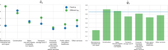
Match efficiency and returns to scale
Compared to our previous results, the match efficiency of “Other Services” increases, while the returns to scale () increase, as shown in Fig. 23. That is, a more congested (high ) labour market leads to fewer matches than other sectors with the same match efficiency and tightness. This reinforces the messages of the MMA: Other Services is a sector that can easily get congested, and a planner seeking to maximise matches taking vacancies as given would move job seekers to more efficient markets which can handle high congestion, like “Construction” or “Sales and Hospitality”.
Rights and permissions
Open Access This article is licensed under a Creative Commons Attribution 4.0 International License, which permits use, sharing, adaptation, distribution and reproduction in any medium or format, as long as you give appropriate credit to the original author(s) and the source, provide a link to the Creative Commons licence, and indicate if changes were made. The images or other third party material in this article are included in the article’s Creative Commons licence, unless indicated otherwise in a credit line to the material. If material is not included in the article’s Creative Commons licence and your intended use is not permitted by statutory regulation or exceeds the permitted use, you will need to obtain permission directly from the copyright holder. To view a copy of this licence, visit http://creativecommons.org/licenses/by/4.0/.
Reprints and permissions
About this article
Cite this article
Carrillo-Tudela, C., Clymo, A., Fuente, C.L. et al. Spanish labour market, mobility and labour shortages. SERIEs (2025). https://doi.org/10.1007/s13209-025-00306-z
- Received
- Accepted
- Published
- DOI https://doi.org/10.1007/s13209-025-00306-z
Keywords
- Job search
- Industry mobility
- Vacancies
- Mismatch
- Labour shortages
JEL Classification
- E24
- J23
- J62
- J63
- J64