Article Content
1 Introduction
Social networks have become ubiquitous, with over 4.5 billion people actively using platforms like Facebook, Twitter, Instagram, and LinkedIn. As these online social platforms continue explosive growth, understanding their complex interconnected structure is increasingly vital for areas ranging from public health to commerce. Online social networks contain a lot of data on social interaction and social relations. Many scholars conduct relevant research on these big data, they have made contributions to relevant field issues such as to resolve spread, society, economy, politics, and so on (Crandall et al. 2008; Romero et al. 2011; Heidemann et al. 2012; Ellison and Boyd 2013; Probst et al. 2013; Berger et al. 2014; Ellison et al. 2014; Ke et al. 2014; Wu et al. 2014, 2017; Grabner-Krauter and Bitter 2015; Chen et al. 2015; Cardoso et al. 2017; Zhong-Ming, et al. 2017; Villota and Yoo 2018).
In an online social network, users can be regarded as nodes of the network; and their attention, recommendations, quote, comments can be regraded as different types of the edge between nodes. Because of the ubiquitous unidirectional features between users such as attention, recommendation, quote, and so on, the online social network, in general, is a directed network, which can be abstract as a directed graph.
Mapping the connectivity within social graphs can identify tightly-knit communities and influential nodes for viral marketing. Harnessing word-of-mouth effects among dense sub-graphs enables targeted, cost-effective promotion diffusion. However, adversaries can also exploit this viral spread for misinformation campaigns. And recommendation systems in e-commerce leverage profiling attributes and underlying social network links to suggest relevant products and services. What’s more, public health policymakers must track infection trajectories during outbreaks based on human contact networks, using analytical network models to predict transmission rates and guide containment strategies. Overlooking super-connector nodes gives rise to risks of escalating epidemics.
In summary, unraveling the intricately tangled web of social interactions is pivotal for security, innovation and responsible community growth. Efficient distributed algorithms to uncover strongly connected components provide actionable insights from relationship big data. Our proposed approach aims to make such analysis computationally tractable.
2 Related work
About the strongly connected component of a directed graph, there are increasingly researchers have contributed to this in recent years, relevant studies can be divided into the following categories:
- 1.SCC decomposition: For example, Bloemen et al. (2016) have studied multi-core dynamic SCC decomposition; Aldegheri et al. (2019) have studied the parametric multi-step scheme of GPU accelerated graph decomposition into SCC; Wijs et al. (2016) have studied the algorithm for graph parallel decomposition into SCC and maximum endpoint component.
- 2.Research on SCC algorithm in different scenarios: For example, Baswana et al. (2019) have studied an algorithm that is effective in the fault-tolerant model; Henzinger et al. (2019) have studied how to calculate two edges and two vertexes in secondary time; Ji et al. (2018) have studied identify SCC in parallel by spanning tree; Pearce (2016) have studied space-efficient algorithm for SCC; Sun et al. (2019) have studied BSP based on federated cloud computing algorithm for SCC. Xu and Wang (2018) and Xu et al. (2020) studied how to calculate the SCC of a simple directed graph. They based their approach on generalized rough set theory. Additionally, they explored searching for the SCC using a granulation strategy; Liao et al. (2019) proposed an efficient algorithm for incremental strongly connected components. This algorithm is designed for dynamic directed graphs. Dahiphale (2023) proposed a distributed and parallel algorithm for identifying 2-edge-connected components (2-ECCs) in large undirected graphs. He also provided a comprehensive analysis of the algorithm’s time complexity.
- 3.Research on SCC and GPU: For example, Li et al. (2017) have studied the high-performance detection based on GPU for sparse graph; Chen et al. (2017) have studied the parallel detection for SCC on coordinate GPU; Devshatwar et al. (2016) have studied the parallel SCC calculate extend centered on GPU; Aldegheri et al. (2019) have studied the multistep scheme of accelerated graph decomposition into SCC; Hou et al. (2016) have studied the multi-partition parallel strongly connected component detection based in GPU; Wijs et al. (2016) have studied the efficient GPU algorithm for graph parallel decomposition into SCC;
- 4.SCC application research: Hongguo et al. (2018) have studied the efficient calculation of page ranking based on SCC. Wiener et al. (2016) have studied named entity parser of AOL and the resolution of disambiguation by document SCC and special edge construction; Wu et al. (2020) have studied the structure controllability of a type of strongly connected complex networks; Zhang et al. (2018) have studied how to use a kind of strongly connected component to achieve efficient directed treatment based on disk; Sowah et al. (2016) have studied the multi-target tracking using SCC;
- 5.Other research categories of SCC: for example, Bernstein et al. (2019) studied the single source accessibility in SCC decline and near-linear time; Chechik et al. (2016) studied decreasing single-source reachability and total SCC update time; Caravelli et al. (2016) studied the appearance of giant strong connected components in spin percolation of continuous media disks; Chatterjee et al. (2018) studied the lower bound of symbolic computation on graphs including SCC, etc.; Kurilic (2015) studied isomorphic SCC; Lu (2021) studies the centrality measure based on hierarchical walking based on the accessibility between SCC in the directed graph; Shekhar et al. (2018) studied SCC cluster solution (SCCC); Attia et al. (2016) studied the re-configurable architecture for detecting SCC;
This paper studies a distributed parallel algorithm for obtaining strongly connected components (SCC) of directed graphs under the background of data distributed storage. It belongs to the second type of research above, that is, research on SCC algorithm in different scenarios. As far as online social network applications are concerned, this is a basic data processing problem.
The classical algorithms for finding the strongly connected components of a directed graph are the Kosaraju algorithm (Sharir 1981) and the Tarjan algorithm (Tarjan 1972).
Since the beginning of this century, many scholars have made their contributions in finding the parallel algorithm for strongly connected components of directed graphs. For example, Mclendon et al. (2005), Barnat et al. (2009), Fleischer et al. (2000), Tomkins et al. (2014, 2015) and Slota et al. (2014) have studied distributed parallel algorithms in the context of multiprocessors. These researches are mainly based on the technology of graph segmentation into independent sub-graphs, that is, a graph is divided into non-interconnected independent sub-graphs, and the segmented sub-graphs continue to be segmented until they cannot be segmented. This method can deploy the solution for strongly connected components in a directed graph on a multiprocessor system. However, it falls under the category of input distributed parallel processing in data sets. This is because it requires a complete graph to be input into the system at the start of the algorithm.
Since Google adopted data distributed storage and the map-reduce processing model (Thusoo et al. 2009), distributed parallel processing has gained prominence. It has become the standard method for data processing in massive data systems. However, the current algorithms for finding the strongly connected components of directed graphs, whether classical algorithms or parallel processing algorithms, do not support this processing method.
This paper presents an algorithm for finding the strongly connected components of a directed graph: interconnected set merging algorithm. It can run independently or in distributed parallel based on the map-reduce data processing model.
3 Basic concepts and terms
is a directed graph, is a set of nodes, and is a set of directed edges. If there are more than two edges from a node to , there is no substantial difference in terms of solving a strongly connected component from the existence of only one edge from to . Therefore, this paper will search for this problem based on a simple directed graph, which means that there is at most only one directed edge from one node in V to another.
Definition 1
Simple directed graphs.
is a simple directed graph, is a set of nodes and is a set of edges. The edges of a simple directed graph can be expressed by an ordered pair: is a directed edge (arc) from to . means directly connect to , and it can be recorded as .
Definition 2
Node connectivity and interconnection.
is a simple directed graph.
(1) The node is connected, and it can be denoted as :
1) Given arbitrarily , (reflexive);
2) If , then (directly connected is connected);
3) If and , then (transitivity).
(2) If and , we call interconnects with , and we denote it as .
Definition 3
The interconnected set, Connectivity and Interconnection of interconnected set.
is a simple directed graph.
(1) ⊂ V. If given arbitrarily exists and it demands , we call is the interconnected set on .
(2) ⊂ are the interconnected sets on . If , exists, we call the interconnected sets is connected, and we denote it as .
(3) ⊂ are the interconnected sets on . If and , we call the interconnected sets is interconnected and we denote it as .
The following properties can be easily deduced by definition mentioned above.
Property 1
is a simple directed graph, and ⊂ are the interconnected sets on .
If , for any given, it requires .
If , for any given, it requires .
Definition 4
Maximal interconnected sets, strongly connected components.
is a simple directed graph.
(1) ⊂ V is an interconnected set on . Given , arbitrarily, if there is no interconnection for , then is a maximal interconnected set on .
(2) is a maximal interconnected set on . , which is the derived sub-graph of , is a Strongly Connected Component (SCC) of .
As long as we obtain the maximal interconnected set of , we can obtain the strongly connected components of by searching for the corresponding sub-graph of the maximal interconnected set.
From Definition 2, it can be easily found that the interconnected relationship of the upper nodes on is equivalent.
Property 2
is a simple digraph. Given arbitrarily , it has the following laws:
Definition 5
Interconnected equivalence classes, Clusters of interconnected equivalence classes.
(1) (regressive);
(2) If and , then (transitivity);
(3) If , then (symmetry).
is a simple directed graph. We call an interconnected equivalence class of . is an identification node of . is the cluster of the interconnected equivalence class on .
Based on the definition of the interconnected equivalence class and Property 2, the following properties can be deduced.
Property 3
is a simple directed graph, and , a cluster of interconnected equivalence classes of , is a division of .
Property 4
is the interconnected equivalence class cluster of . The connectivity relation of the upper node on (equivalent to the maximum interconnected set of ) is a partial order relation, that is, for any given :
(1) (reflexive);
(2) If and , then (anti-symmetric);
(3) If and , then (transitivity).
Property 5
is a simple directed graph. And the following statements are equivalent.
(1) is a maximal interconnected set of on ;
(2) is an interconnected equivalence class on .
4 Algorithm principle
4.1 Introduction of algorithm
According to Definition 2, the search algorithm for the strongly connected component (SCC) of a directed graph is equivalent to the search algorithm for the derived subgraph of a maximally-interconnected set. According to Property 4, the connecting relation of maximal interconnected sets is a partial order relation. The classic Tarjan algorithm uses a depth-first search strategy. Its essence is to find the maximally interconnected set at the “deepest level” in the partial order relation, which corresponds to the graph. We then use the remaining “map” after “pruning” to continue searching for the “deepest” maximal interconnected set. This process continues until the remaining “map” is empty. The first output of the Tarjan algorithm is based on the global data of the figure, and it is a distributed algorithm.
The mergence algorithm of the interconnected set introduced in this paper follows the depth-first search strategy of the Tarjan algorithm, but takes into account the following facts:
In the case of distributed data storage, although we cannot obtain the maximum interconnected set of the graph (global maximum interconnected set), we can obtain the local maximum set (the interconnected set that cannot be further expanded under distributed data).
In short, the algorithm can be executed into two phases:
Map phase: Obtain the local maximum interconnected set based on the data on the distributed data server, and this process can be distributed and parallel on different servers;
Reduce phase: The calculation results of the Map phase are merged, and the global maximum interconnected set is obtained from the local maximum interconnected set.
To some extent, this algorithm can be regarded as the improvement of the Map-reduce data processing model based on the Tarjan algorithm.
4.2 Algorithm principle
Definition 6
is a simple directed graph.
is the set cluster of the interconnected set on G. If is a division of , we call to be the standard set cluster of the interconnected set on G.
In essence, the algorithm introduced in this paper merges the interconnected sets in the standard set cluster on without breaking the standardization of the set cluster. There are some lemmas as follows.
Lemma 1
is a simple directed graph.
(1) is the interconnected set of on , and is the interconnected set of on if .
(2) is the standard interconnected set cluster on , and if and , then is the standard interconnected set cluster on .
(3) is the standard interconnected set cluster on , and we merged the interconnected set in according to rule (2):
Doing this until this process cannot continue, that is, for any given, no has interconnected, then is the interconnected equivalent class cluster of (maximum interconnected set cluster).
Proof
- (1)According to property 1, any node in is interconnected with any node in . is an interconnected set, and their internal nodes are also interconnected. Therefore, all nodes in the are interconnected.
- (2) is an interconnected set according to (1). Therefore
is the interconnected set cluster on . is standardized, and is the division of . Therefore, is the division of . is the standardized interconnected set cluster on .
- (3)It is known from being the standard interconnected set cluster on and (2) that for any given , is the standard interconnected set cluster on and is the standard interconnected set cluster on and any two of the interconnected sets on are not interconnected. There is only one possibility, that is is the cluster of the maximum interconnected set on .
5 Algorithm
5.1 The organization of graph data on the internet
A Web page can be regarded as a node on the Web, and a link on the Web page defines the edge of that node to another node. In Google Web data storage system, data is organized according to web pages, that is, nodes, which can be abstractly regarded as binary groups:
where is the IP address or URL of the web page,
is the IP or URL of all links on the web page. The binary group (4-1) completely describes the link relationship between web pages (the direct connection relationship between web page nodes—web page link diagram).
Similarly, data from Twitter and Facebook can also be viewed as a set of binary groups (4-1). It’s just that nodes become user ids, and become collections of related user ids like concerns, recommendations, references, and so on.
For a variety of reasons, organizing relational data in Internet systems by nodes is by far the most effective method. The method of relational data organization is equivalent to the relational matrix representation of graphs in graph theory.
5.2 Data organization of the algorithm
5.2.1 Input and output
The set of the binary group (4-1) can represent the connectivity relation between the nodes of the directed graph, but it cannot represent the connectivity relation of the interconnected set. Therefore, we modify (4-1) as:
Here is the identification node of the interconnected set, and is the node-set of the interconnected set, and is the set of identification nodes connected by the interconnected set.
At the beginning of the algorithm, this set is:
In other words, each node in (4-1) is regarded as a single node interconnected set.
Map-reduce is a data processing model usually built on “external storage”. The related algorithms can be called “external algorithms”, which means, the algorithms are based on and using “external memory” (Chen et al. 2017).
The interconnected set union algorithm studied in this paper belongs to the “external algorithm” in its application field. Its features are:
- 1.The input of the Map process is the data on the local data distribution server (external memory);
- 2.The output of the Map process is stored on the local data distribution server and aggregated to the Reduce server after the Map process is completed. Due to datum size, datum collected on the Reduce server is also stored in the Reduce server’s external storage firstly.
- 3.In view of the 2 points mentioned above, the Reduce process is also a process based on and utilizing “external storage”.
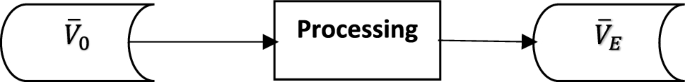
The Fig. 1 shows the data processing process of the algorithm: the interconnected sets are read (searched) one by one and processed until a maximum interconnected set is obtained; Then output (add) the obtained maximum interconnection to . After the output of one maximum interconnection is complete, continue the previous process until all interconnections in are processed.
Reduce processes
5.2.2 Association with distribution calculation and the external suspension
In the Map phase, the algorithm works for datum on the local server, so there may be and that is not in the interconnected sets of . In the Map phase, cannot be processed. is the identifier node of the suspended connected interconnected set , or the suspended connected node of for short.
Suspended state means that the current calculation process is not processed until a subsequent process is completed.
5.2.3 Interconnected set connected chain (stack)
What discussed above describes the input/output data structure of the algorithm, and the following describes the (in-memory) data structure of the algorithm’s intermediate calculation results.
This algorithm follows the depth-first search strategy of the Tarjan algorithm. Through a structure stack (Fig. 2):
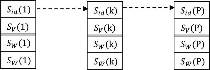
One-way directly connected chain (stack) of interconnection
We can manage a unidirectional directly connected chain (non-loop) of an interconnected set. ,they are the identifier (node) of the interconnected set k of the stack, the node-set, the unprocessed externally connected identifier set, and the extern connected identifier result set, respectively. And P is allied a pointer to the top of the stack (end of the chain) position.
The algorithm ensures that the in-stack (on-chain) items satisfy the following properties.
(1-1) means that the direct connection relationship between the interconnected set on the chain and its direct successor interconnection has been processed;
(1-2) means that the direct connection relationship between the interconnected set on the chain and its direct successor interconnected set is uniformly treated as the relationship between nodes identified by them;
(2-1) and (2-2) mean that there is no (known) direct connectivity between any interconnected set on the chain and its precursor interconnected set (including direct and indirect precursors). This property also holds when k = r. This situation means that the connectivity between nodes in the interconnected set has been eliminated.
The interconnected set connected chain satisfying the above properties has the following properties:
Each interconnected set in the chain has a directly connected relationship with its direct successor interconnected set, and there is no (known) direct connected relationship with its predecessor interconnected set.
5.3 Algorithm explanation
Assume that the current connectivity chain of the interconnected set is as shown in Fig. 2 and satisfies the property (4-5). It processes the external connectivity identifier for the item at the top of the stack (at the end of the chain), which is equivalent to the deep search of the direct connectivity relation of the interconnected set.
If the interconnected set at the stack top unprocessed external connectivity identifier satisfies
it means all external connectivity labels of the top stack interconnected set are processed, and the top stack interconnected set is removed from the stack. When
according to the depth-first search strategy, an external connected identity is obtained
When it comes to , there are three cases:
(I) There is an unprocessed interconnected set , ;
(II) a processed interconnected set exists, like , ;
(III) is a suspended node, that is, for any , .
5.3.1 Case (I) solution
Let’s first look at the solution of case (I). Figure 3 illustrates how to find an unprocessed interconnected set through . are respectively the identity (node) of the interconnected set N, the node-set and the externally connected identity set.
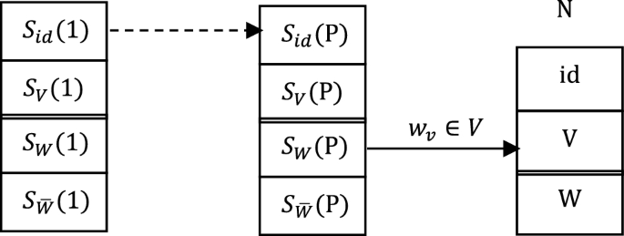
Finding the unprocessed interconnected set N through
Figure 3 reflects the direct connection between the interconnected set at the top of the stack and N, that is . According to the depth-first search strategy, N will be pushed onto the stack.
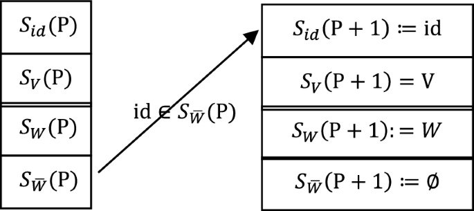
Figure 4 shows the processing before N is pushed on the stack. Item 4 records the direct connection between the interconnected set on top of the stack and the interconnected set N to be pushed on the stack, and uniformly expresses it as:
in order to avoid different representations of direct connectivity of interconnected sets.
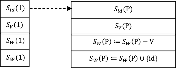
Processing of the interconnected set at the top of the stack before pushing N onto the stack
is a set of interconnections, and is a set of nodes of , maybe a set of multiple nodes, and they reflect the same direct connection relationship . This relationship has been confirmed by , so item 3 is not but .
Figure 5 shows the process of pushing onto the stack. After pushing onto the stack, the connecting chain of the interconnected set still retains the properties of (1-1) and (1-2) in (4-5).
N is put onto the stack
The post-push processing is not finished after is put onto the stack, and the loop on the connected chain of the interset needs to be eliminated. Figure 6 shows loop detection.
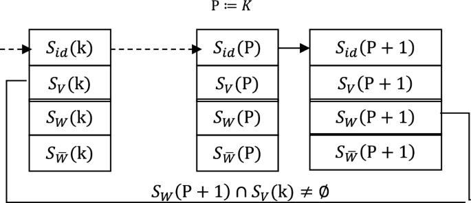
Loop detection after pushing N onto the stack
Compare from the beginning
until the first satisfies the condition is found. Thus a (maximum) loop is found on the connected chain of the interconnection:
According to Lemma 1, all interconnected sets on a loop are interconnected and can be combined into one interconnected set. Figure 7 illustrates the process when the loop merges. After the loop merges, the pointer on the top of the stack is:
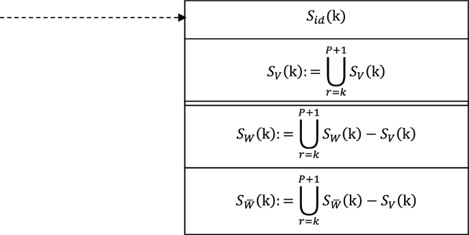
Loop merge
5.3.2 Case (II) solution
If case (I) is not satisfied, that is, there is no unprocessed interconnected set , to satisfy the condition that . We must first make sure whether it satisfies the case (II). If there is an interconnected set that has been processed, then only the operation as shown in Fig. 4 is needed to determine the direct connection relationship between the interconnected set S(P) and N on the top of the stack, and N does not need to be pushed (repeatedly) onto the stack.
5.3.3 Case (III) solution
If neither (I) nor (II) is satisfied, is a suspended node and will be transferred from to
In case the Reduce process continues.
5.4 Algorithm description
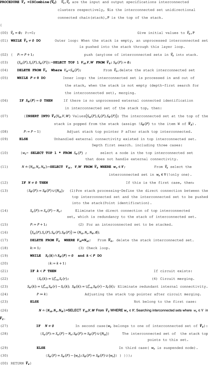
Because SQL language is more convenient to describe the operation of a multivariate group set, we use pseudo code that is similar to C-SQL to describe the algorithm. The following is a description of some special syntax in pseudo-codes.
In lines (03), (10), (11), (26) of the algorithm’s pseudo-code, we assign the result of the Select to a tuple or variable, where the tuple is enclosed in parentheses for clarity, line (11):
“” is read as ” defined as “. The result of Select is usually a set of tuples, but can also be tuples and variables, so (4-6) can also be regarded as a set of unit groups, and in (12) will be regarded as a set of unit groups.
Select in line (03) and (10) means the first tuple that satisfies the condition.
In the algorithm description, the input and output , of the algorithm are regarded as a special relationship with 3 properties named (with set properties), where is the identification node of the interconnected set, V is the node-set of the interconnected set, and is the identification node set of the interconnected set directly connected by the interconnected set.
For intuitive representation, all data items involved in the set in the algorithm are regarded as a “pseudo relationship” and queried by Select. For example, row (10):
means taking an element from the top of the stack into . Therefore, and cannot exit the stack separately, so case (5) is not true.
The C-SQL pseudo code of the algorithm is described as follows:
5.5 Experiments
5.5.1 Experimental purpose
Validate the efficiency and performance improvement of the proposed Map Reduce algorithm in finding strongly connected components in directed graphs, and conduct statistical analysis to evaluate the significance of the results.
5.5.2 Experimental environment
We conducted our experiments on a Hadoop cluster consisting of 10 nodes, each with 16 GB of RAM and Intel Xeon processors. The implementation was done using Apache Hadoop version 2.9.2 and Java version 8.
5.5.3 Graph generation
We utilized synthetic benchmark graphs generated using the Barabási–Albert model for scale-free networks and the Erdos–Renyi model for random graphs. The parameters for these models were set to ensure a variety of structures: for the Barabási–Albert model, we used a parameter m = 3 to control the number of edges added from a new vertex to existing vertices. For the Erdos–Renyi model, we varied the edge probability p to create graphs with different densities. Specifically, we tested probabilities of p = 0.1, 0.05, 0.01. The data-set encompasses graphs of varying scales, including small (thousands of nodes), medium (tens of thousands of nodes), and large (millions of nodes) graphs. In our experimental setup, we partition the graph datasets of different sizes into training and testing sets. We utilize standard strongly connected component algorithms, such as Kosaraju’s algorithm or Tarjan’s algorithm, as benchmarks to compare the results.
5.5.4 Data format and storage
The input data will be stored in an edge list format, where each line represents a directed edge in the format of “source_node target_node.” The following example illustrates edges from node 1 to node 2, from node 2 to node 3, from node 3 to node 1, and from node 4 to node 3:
- 1.2
- 2.3
- 3.1
- 4.3
Each line denotes a directed edge. The data can be stored in text files on servers, with the input data uploaded and stored in HDFS (Hadoop Distributed File System). To optimize read performance, the data is divided into multiple blocks, with a default block size of 128MB (which can be adjusted as needed). Each block contains several lines of edges. HDFS automatically partitions files into blocks, allowing for parallel reading of data in a distributed environment, thus enhancing overall processing speed.
5.5.5 Data partitioning scheme
We have designed a data partitioning strategy to ensure efficient allocation of input data to various mappers. The steps for data partitioning are as follows:
- 1.Data Loading: Load the edge list data from HDFS using the ‘FileInputFormat’ class of the Mapper API to read the input files.
- 2.Hash Partitioning: A hash function is applied to the source node of each edge to distribute the data across different mappers. For example, the hash value can be determined using ‘hash(node_id) % num_mappers’ to allocate edges to specific mappers. This approach ensures that different source node IDs map to different mappers, promoting uniform data distribution.
- 3.Input Partition: Each mapper is responsible solely for the edges it receives, storing them in local memory for subsequent processing. For example, if there are four mappers, the partitioning of edges for each mapper would be as follows:
Mapper 1: Handles all edges where ‘hash(node_id) % 4 = = 0’
Mapper 2: Handles all edges where ‘hash(node_id) % 4 = = 1’
Mapper 3: Handles all edges where ‘hash(node_id) % 4 = = 2’
Mapper 4: Handles all edges where ‘hash(node_id) % 4 = = 3’
5.5.6 Determining the number of mappers
To fully leverage parallelism, it is essential to determine an optimal number of mappers. This begins with an assessment of computational resources, evaluating factors such as the number of CPU cores and memory size available on the server to determine the resources allocable to each mapper. For example, if a server has eight CPU cores, a feasible setting can be between four and eight mappers. Following this, experimental evaluation is conducted, testing different quantities of mappers (e.g., 4, 8, 12) and recording processing time and resource utilization. Experiments will also be conducted using randomly generated directed graphs of varying scales (1 million to 10 million edges) across different datasets. The goal is to identify the number of mappers that produces the shortest processing time and the best CPU/GPU utilization. The number of mappers will be increased incrementally, observing the impact of these changes on algorithm performance to find the optimal configuration.
5.5.7 Addressing bottlenecks with a single reducer
Using a single reducer for all mappers can result in performance bottlenecks. To address this issue, we implement multiple reducers and devise a method to distribute the reduce tasks across these reducers using appropriate keys for partitioning. For instance, different strongly connected components can be assigned to different reducers. Moreover, we adopt a staged processing approach: initially, the data is processed in parallel by multiple mappers to obtain local strongly connected components. These local results are then passed to one or more reducers for merging. The reducers will combine the data corresponding to the same key (i.e., the same strongly connected components), progressively generating the final output of strongly connected components.
5.5.8 Data-set and cluster sizes
We generated graphs ranging in size from 1000 to 10,000 vertices and 10,000 to 1,000,000 edges to evaluate the algorithm’s performance with varying data-set sizes. Additionally, we tested the algorithm on clusters with different configurations, ranging from 2 to 10 nodes, to visualize the impact of node count on performance.
5.5.9 Algorithm implementation and evaluation
We implemented the proposed Map-Reduce algorithm and executed it in a Hadoop cluster environment. Each run’s execution time was collected, and resource consumption metrics (such as memory usage and CPU load) were recorded. The execution involved running the algorithm multiple times on various datasets (e.g., five times) to obtain stable performance data. For each experimental setup, we recorded the algorithm’s runtime and the number of strongly connected components (SCCs) identified.
Performance Metrics: We evaluated our algorithm’s performance using several key metrics:
Execution time: Measured in seconds, representing the total time taken from initiation to completion.
Memory usage: Monitored to ensure that the algorithm operates within acceptable resource limits.
Scalability: Assessed by determining how execution time and memory usage change with respect to increasing graph sizes and varying the number of nodes in the cluster.
Accuracy: Verified by cross-referencing the identified strongly connected components with those obtained from a depth-first search (DFS) implementation on the same graphs.
Statistical Analysis: The average execution time and standard deviation for each set of experiments were calculated, along with a 95% confidence interval. Statistical tests were conducted to compare the execution times of the Map-Reduce algorithm against the baseline algorithm. The experimental data were compiled to contrast the performance of the Map-Reduce algorithm and the baseline algorithm across different graph sizes, leading to a statistical analysis (Table 1). The results of the experiments are summarized as follows:
In the small graph category, the execution time of the Map-Reduce algorithm was significantly lower than that of the baseline algorithm, with an average time representing only 20% of the baseline. The confidence interval indicates that the results are stable and reliable. In both medium and large graph categories, the advantages of the Map-Reduce algorithm were even more pronounced, with execution times significantly below those of the baseline algorithm; p values of less than 0.01 indicate statistical significance. These results demonstrate that as the graph size increases, the efficiency advantage of the Map-Reduce algorithm becomes increasingly evident.
5.5.10 Empirical conclusion
The experimental results confirm the significant efficiency improvements of our proposed Map-Reduce algorithm for identifying strongly connected components in directed graphs. The statistical analysis enhances the reliability of the results and suggests that future research should explore the optimization of algorithms and their application to other types of graphs. Moving forward, we aim to further optimize the algorithm based on the experimental outcomes, test it on more diverse graph datasets, and investigate how various parameter settings influence performance, with the goal of enhancing the efficiency of SCC identification.
6 Algorithm proof
6.1 Properties of the algorithm
Lemma 2
The input of the algorithm is the standard interconnected cluster of G, ,, and if directly connected to (–), that is to say, Vq , then will not precede the stack compared to .
Proof
The following lists all possible push () and pull () orders for and .
- 1.
- 2.
- 3.
- 4.
- 5.
- 6.
According to the stack processing rules, (3) and (6) will not occur. (1) and (5) need to be excluded.
First, let’s look at (1). Only when is the interconnected set at the top of the stack can it be possible for to exit the stack. Let’s assume the current top interconnection
According to case (1), has not been pushed onto the stack (). According to the propositional condition , that means, exists to satisfy . The top stack interconnected set does not leave the stack until the processing is completed. And the processing will result in being pushed onto the stack, that is, the push of will precede the exit of . So, case (1) is not true.
According to case (5), when is pushed on the stack, is in the stack. Because connect directly to , the interconnected loop detection-merge process of the algorithm will merge and into . Therefore, and cannot exit the stack separately, so case (5) is not true.
There are only two cases left: (2) and (4). In both cases, exit the stack later than .There are only two cases left: (2) and (4). In both cases, exit the stack later than .
The End.
An immediate consequence of Lemma 2 is as follows.
Corollary 1
If is connected to , that’s to say , will not exit the stack earlier than .
Proof
, so, there must be
According to Lemma 2, will not exit the stack earlier than , and will not precede ,…, will not precede , so does not precede to exit the stack.
The End.
Here are the inferences.
Corollary 2
, if interconnected with each other ( and ), then all nodes in and will exit the stack at the same time (they are merged to the same interconnected set).
Proof
According to Corollary 1, will not exit the stack earlier than , will not exit the stack earlier than . Then there is only one possibility: all nodes in and (merged into the same interconnection) will exit the stack at the same time.
The End.
Delete ((04), (17)) from when the interconnected set is pushed onto the stack, and put ((07)) onto the stack when the top interconnected set is being moved from the stack. When the algorithm runs for the time , all interconnected sets are distributed in (t), (t) and stack . Let
Lemma 3
is the representation of the direct connectivity relation between the standard interconnected set cluster and its belonging interconnected set. For any given , is the representation of the direct connectivity relation between the standard interconnected set cluster and its belonging interconnected set.
Proof
can only be changed in the algorithm in one case, that is, interconnected sets are merged ((22)). And the premise of the union of interconnected sets is that the merged interconnected sets are interconnected. According to Lemma 1(2), this does not change the normalization of .
is standard. And for any given , it is standard.
The following instructions explains that fully represent the direct connectivity of the interconnected sets.
- 1.Before the interconnected set is pushed onto the stack, the information that is recorded in the external connectivity identification result set of the interconnected set on the top of the stack (Fig. 3 and Algorithm description (14)). The push of does not break the property represented by the direct connectivity of the interconnection .
- 2.When the interconnected set is combined, the directly connected items and outside the interconnected set are merged at the same time (Fig. 6 and algorithm description (22–23)). The merging of interconnected sets does not break the properties represented by the direct connectivity of interconnection .
- 3.For the interconnected set that has been completed and moved out of the stack, the algorithm also carries out reservation processing for the directly connected items of (algorithm description (28)).