Article Content
Abstract
On December 27, 2022, the Spanish government announced a temporary value added tax (VAT) rate reduction for selected products. VAT rates were cut on January 1, 2023. Initially, the VAT was expected to go back to their previous level six months later, but several waivers led this policy to last for 21–24 months, where the VAT returned to its original level in two phases. We study the pass-through of the temporary VAT rate changes covering the daily prices of roughly 21.000 food products sold online in a Spanish supermarket. We achieve this by utilizing a dataset obtained by web-scraping and employing machine-learning methods to classify each product into a COICOP5 category. To identify the causal price effects, we compare the evolution of prices for treated items (that is, subject to the tax policy) against a control group (food items out of the policy’s scope). Our findings indicate that, at the supermarket level, the pass-through was almost complete after one week. In using product characteristics, we notice differences in the rate of pass-through and in pricing strategy in the subsequent weeks.
Explore related subjects
Discover the latest articles and news from researchers in related subjects, suggested using machine learning.
- Analysis
- Consumer Behavior
- Market Intelligence
- Microeconomics
- Policy Implementation
- Policy Evaluation
Notes
-
Utilizing scanner data raises some concerns as regards the aggregation process, and micro-CPI data collected by National Statistical Offices might introduce bias, due to the collection of data via sampling and as products are censored and replaced. This may affect some estimations. For more details on the pros and cons of these data see Cavallo (2018).
-
To accurately consider price variations arising from quality differences, it is essential to compare prices using consistent units. As we have the quantities detailed in the description, we can determine the unit price. However, we investigate how products that are less expensive overall yet have a higher unit price impact purchasing decisions. Consequently, our emphasis is on the total expenditure required to purchase a particular product. For example, comparing 5 L of olive oil with a 200-ml bottle, the latter may appear costlier when evaluated in standardized units, such as euros per liter.
-
For more details about the PRISMA network run by the ECB see link which is a follow-up of the “Inflation Persistence Network” (IPN).
-
Datamarket is a company which offers web-scrapped datasets on many topics, for more information see here.
-
We target the Classification of individual consumption by purpose (COICOP) classification by (1) division (two digit), (2) group (three digit), (3) class (four digit), (4) sub-class (five digit) and (5) product.
-
Several initiatives are in place, but still the resources needed, both in terms of human capital and computation, are immense. As an example, the “Project Spectrum” is a joint project that reflects this need and will encompass the product classification for more supermarkets and retailers, as well as other products sold in other types of stores different from food in supermarkets. For more details, see “Project Spectrum: using generative AI to enhance inflation nowcasting”.
-
For more details, see Box 1 Price setting in Germany in the light of the temporary value added tax cut in 2020: evidence from micro-price data. They found that the price reaction to the VAT cut was quick and substantial.
-
They make use of the supermarket prices collected by Datamarket, a private initiative.
-
For more details on the DPD dataset see box 3 “The ECB Daily Price Dataset” in Strasser et al. (2023).
-
The original dataset contains also information on beverages, cleaning supplies, small electronic appliances and personal care products. Due to the nature of this paper, we take them out of the sample.
-
GTIN-EAN 13 digit is the identifier of a unique product which harmonized and used by the super-markets. This identifier allows us to proxy imported products versus domestic products.
-
Another approach would be to use the classification used by the shop as in Eichenbaum et al. (2011), but this would prevent us from comparing with the official data and would pose some difficulties in comparing between different retailers as they do not follow the same criteria.
-
Harmonized Index of Consumer Prices.
-
Given that some products life span is very short and that can bias this calculation. We remove products whose prices are available for a short period of time.
-
It is important to point out that for product spells with identical duration, calculating the frequency of price changes will yield the same result whether done on an individual product basis with a subsequent averaging or by calculating the proportion of price changes on a specific date and then averaging across products. In contrast, when the durations of time spells vary between products, such computation could introduce a bias.
-
We opt for this specification rather than the usual one found in pass-through literature where the dependent variable is the price change (∆pit), to prevent occurrences of zeros since products might not update their prices often.
-
We suspect this is due to the holiday season where the non-treated goods by the VAT measure registered some differentiated price-setting dynamics.
-
Log-lin model coefficient interpretation: Effect = exp(β) − 1.
-
GTIN stands for Global Trade Item Number. This is a 13-digit code, the first two or three digits are the country code. Note that this is a proxy, as sometimes multinationals register in different locations from the production location for some reason.
-
For more details on the use of scanner data in constructing official CPI statistics see https://www.ine.es/metodologia/t25/ipc_scanner_data.pdf.
-
For more details on the Spanish INE micro-CPI data, see https://assets.aeaweb.org/asset-server/files/21477.pdf.
-
We target the Classification of individual consumption by purpose (Coicop) classification https://ec.europa.eu/eurostat/statistics-explained/index.php?title=Glossary:Classification_of_individual_consumption_by_purpose_(COICOP) by (1) division, (2) group, (3) class, (4) sub-class (to give an example, this would be”01.1.1—Rice”) and (5) product.
-
We use 2023 CPI weights by 5-digit issued by the Spanish statistical office (check this here).
-
The exception is for the ensemble machine-learning algorithm model we propose to evidence that our preferred method outperforms this and other method, in which we run a classical text processing pipeline.
-
Tokens are groups of characters, which sometimes align with words, but not always. For instance, our “Pizza” product description contains precisely 20 tokens.
-
This mechanism is also behind some famous models such as ChatGPT.
-
We use this model.
-
Learning rate of 3e-5, batch size of 8 and 20 epochs, with resulted on an average of 0.92% F1-score over the threefold subsets.
-
An extra label or category is added: non-food products.
-
These were: All features, log and 300 trees.
References
-
Almunia M, Martínez J, Martínez Á (2023) La reducción del iva en los alimentos básicos: evaluación y recomendaciones. EsadeEcPol Brief. https://doi.org/10.56269/20230328
-
Amores AF, Barrios S, Speitmann R and Stoehlker D (2023a) Price Effects of Temporary VAT Rate Cuts: Evidence from Spanish Supermarkets. JRC Research Reports, JRC132542, Joint Research Centre (Seville site). https://ideas.repec.org/p/ipt/iptwpa/jrc132542.html
-
Ash E, Hansen S (2023) Text algorithms in economics. Ann Rev Econ 15(1):659–688
-
Basso HS, Dimakou O and Pidkuyko M (2023) How inflation varies across Spanish households. Occasional Papers, 2307, Banco de Espan˜a. https://doi.org/10.53479/29792
-
Benzarti Y, Garriga S and Tortarolo D (2022) Can vat cuts dampen the effects of food price inflation? Working paper. https://dtortarolo.github.io/WebPage/VAT_inflation.pdf
-
Bernardino T, Gabriel RD, Quelhas J and Silva-Pereira M (2024) The full, persistent, and symmetric pass-through of a temporary vat cut. mimeo. https://www.ricardoduquegabriel.com/files/BGQS_2024.pdf
-
Burstein, Ariel, and Gita Gopinath. (2014). International Prices and Exchange Rates, vol. 4. Elsevier, pp. 391–451. Preliminary January 2013. Prepared for the Handbook of International Economics, Vol. IV. https://doi.org/10.1016/B978-0-444-54314-1.00007-0
-
Campbell JR, Eden B (2014) Rigid prices: evidence from u.s. scanner data. Int Econ Rev 55(2):423–442. https://doi.org/10.1111/iere.12055
-
Cavallo A (2013) Online and official price indexes: measuring argentina’s inflation. J Monetary Econ 60(2):152–165. https://doi.org/10.1016/j.jmoneco.2012.10.002
-
Cavallo A (2017) Are online and offline prices similar? Evidence from large multi- channel retailers. Am Econ Rev 107(1):283–303
-
Cavallo A (2018) Scraped data and sticky prices. Rev Econ Stat 100(1):105–119. https://doi.org/10.3386/w21490
-
Cavallo A, Gopinath G, Neiman B, Tang J (2021) Tariff pass- through at the border and at the store: evidence from us trade policy. Am Eco- Nomic Rev: Insights 3(1):19–34. https://doi.org/10.1257/aeri.20190536
-
Devlin J, Chang M-W, Lee K and Toutanova K (2019) Bert: Pre- training of deep bidirectional transformers for language understanding. 54
-
Eichenbaum M, Jaimovich N, Rebelo S (2011) Reference prices, costs, and nominal rigidities. Am Econ Rev 101(1):234–262. https://doi.org/10.1257/aer.101.1.234
-
Fuest C, Neumeier F, Stöhlker D (2025) The pass-through of temporary VAT rate cuts: evidence from German supermarket retail. Int Tax Public Financ 32(1):51–97
-
Gagnon E (2009) Price setting during low and high inflation: evidence from Mexico*. Q J Econ 124(3):1221–1263. https://doi.org/10.1162/qjec.2009.124.3.12217
-
Garc´ıa-Miralles E (2023) Support measures in the face of the energy crisis and the rise in inflation: an analysis of the cost and distributional effects of some of the measures rolled out based on their degree of targeting. Economic Bulletin. https://api.semanticscholar.org/CorpusID:257395075
-
Gautier E, Marx M, Vertier P (2023) How do gasoline prices respond to a cost shock? J Polit Econ Macroecon 1(4):707–741. https://doi.org/10.1086/727698
-
Gautier E, Conflitti C, Faber RP, Fabo B, Fadejeva L, Jouvanceau V, Menz JO, Messner T, Petroulas P, Roldan-Blanco P, Rumler F (2024) New facts on consumer price rigidity in the euro area. Am Econ J: Macroecon 16(4):386–431. https://doi.org/10.1257/mac.20220289
-
Hansen S, Lambert PJ, Bloom N, Davis SJ, Sadun R, Taska B (2023) Remote work across jobs, companies, and space. Natl Bur Econ Res. https://doi.org/10.3386/w31007
-
Henkel L, Wieland E, Błażejowska A, Conflitti C, Fabo B, Fadejeva L, Jonckheere J, Karadi P, Macias P, Menz JO, Seiler P (2023). Price setting during the coronavirus (COVID-19) pandemic. Occasional Paper Series, 324, European Central Bank. https://ideas.repec.org/p/ecb/ecbops/2023324.html
-
Kehoe P, Midrigan V (2015) Prices are sticky after all. J Monetary Econ 75:35–53. https://doi.org/10.1016/j.jmoneco.2014.12.004
-
Lafrogne-Joussier R, Martin J, Mejean I (2023). “Cost pass-through and the rise of inflation”. mimeo. http://www.isabellemejean.com/lmm_ppi_v2.pdf
-
Lehmann E, Simonyi A, Henkel L and Franke J (2020) Bilingual transfer learning for online product classification. In: Proceedings of Workshop on Natural Lan- guage Processing in E-Commerce. Association for Computational Linguistics, pp. 21–31. https://aclanthology.org/2020.ecomnlp-1.3
-
Montag F, Sagimuldina A and Schnitzer M (2020) “Are temporary value- added tax reductions passed on to consumers? Evidence from germany’s stimulus”.
-
Nakamura E, Steinsson J (2008) Five facts about prices: a reevaluation of menu cost models. Q J Econ 123(4):1415–1464
-
Amores AF, Basso HS, Bischl JS, De Agostini P, Poli SD, Dicarlo E, Flevotomou M, Freier M, Maier S, García-Miralles E, Pidkuyko M, Ricci M and Riscado S (2023b) In- flation, Fiscal Policy and Inequality. ECB Occasional Paper No, 2023/330, European Central Bank. https://doi.org/10.2139/ssrn.4604418
-
Reimers N, and Gurevych I (2019) Sentence-bert: Sentence embeddings using siamese bert-networks. 5, 51, 56
-
Sanh V, Debut L, Chaumond J, Wolf T (2020). Distilbert, a distilled version of bert: smaller, faster, cheaper and lighter. 5, 11, 54, 55
-
Strasser G, Wieland E, Macias P, B±açzejowska A, Szafranek K, Wittekopf D, Franke J, Henkel L, Osbat C (2023). E-commerce and price setting: evidence from Europe. Occasional Paper Series, 320, European Central Bank. https://ideas.repec.org/p/ecb/ecbops/2023320.html 9
-
Tunstall L, Reimers N, Jo UE, Bates L, Korat D, Wasserblat M, Pereg O (2022). Efficient few-shot learning without prompts. 5, 56
-
Vaswani A, Shazeer N, Parmar N, Uszkoreit J, Jones L, Gomez AN, Kaiser L and Polosukhin I (2023) Attention is all you need. 53
-
Wooldridge, Jeffrey M. (2021). Two-way fixed effects, the two-way mundlak regression, and difference-in-differences estimators. Available at SSRN 3906345. 20
Acknowledgements
We are deeply grateful to the anonymous referee for their thorough and insightful feedback, which significantly enhanced the quality and rigor of this manuscript. We also thank Erwan Gautier (Banque de France) and Aitor Lacuesta (Banco de Espan˜ a) for their valuable comments and guidance. We are especially grateful to the Daily Price Dataset (DPD) Team at the ECB for making available these data for research purposes and for guiding us. The authors also thank Datamarket for sharing the data set with us. The opinions and analyses are the responsibility of the authors and therefore do not necessarily coincide with those of the Banco de Espan˜ a or the Eurosystem. This research was conducted during a secondment at Banque de France (BdF) under the External Working Experience program. The hospitality of the Banque de France and especially of the Service de Études Microéconomiques is gratefully acknowledged.
Additional information
Publisher’s Note
Springer Nature remains neutral with regard to jurisdictional claims in published maps and institutional affiliations.
This research was conducted during a secondment at Banque de France (BdF) under the External Working Experience program. The hospitality of the Banque de France and especially of the Service des Analyses Microéconomiques (SAMIC) is gratefully acknowledged.
Appendices
Appendix
Data on prices online
2.1 Data Cleaning and treatment
To make the microdata suitable for our purposes, we implemented a number of methodological interventions to deal with missing observations, sales and promotions, and other features of daily web-scraped data. Include, the number of prices available on a daily basis from each retailer are shown in Fig. 18.
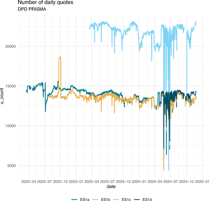
Source: DPD Prisma. Number of observed prices on a daily basis by retailer and shop. Not filtered nor classified
Daily number of products (raw data).
Data cleaning and price filling. We drop observations that are clearly errors (such as exorbitant prices) and exclude price changes smaller than 0.1%, as well as increases above 100.0%, to account for possible measurement error. We get rid of those products for which the number of observations is below a certain threshold of day, calculated as the number of observations out of the maximum number of possible daily observations (for DPD Prisma this is from the 1st of April 2022 up to October 2024). The sequence of price records can be interrupted because (i) it reaches the end of the observation period, (ii) an item is out-of-stock (temporally or permanently), or (iii) a technical issue (e.g., robot(s) and/or website(s) go offline). These instances can affect the length of price spells, most likely shortening them. If we observe missing observations for a certain amount of days, (21 days), these are filled forward with the most recent usable price and replace the unusable or missing observation to fill in the gaps. We assume that these short gaps are related with a problem with the scraper that collects the data that led to web-scraping routine failures, rather than stock outs, as in the case of miss-reporting the failure would be broad-based. This new price series are labeled as filled series.
Sales filter. Since the price information includes temporary sales and promotions, and that can alter the results of some of the statistics. We filter the series to account for temporary sales to eliminate the high frequency of price changes. A temporary sale is defined as prices that remain below the usual price and return to its previous level, we allow for a time window below 21 days (we use the filter proposed by Nakamura and Steinsson, (2008)) and we also filter temporary increases, also for 21 days (here we use the filter proposed by Kehoe and Midrigan (2015)). In some specific cases, retailers show a particular pricing behavior, so we relax the condition where the criteria allow for small changes within a bracket instead of the condition that the price has to return to the previous level. This observed pattern of not returning to the previous price seems to be related with certain characteristics of a particular establishment that mainly operates in large cities.
We have an unbalanced panel as some product items are not always available or have missing price information.
On the entry and exit of products. For a limited number of products we observe product churning. So we impose some continuity by restricting the sample to those products whose price is observed for a long period of time. We remove products that are observed for less than 100 days.
In general, we have used DPD Prisma on a daily frequency. But in some cases, we explore the results using the data on a weekly frequency. In this circumstance, we can take the last observation, the mean, or the mode of a given week. As we want to explore the implications of the bias due to mean averaging, we use the mean.
Product Grouping. To classify the products, we have used the following strategies:
- Processed and unprocessed foods: We classify the products according to Coicop4 class.
- Trademark and white label: We extract the label of each product from the description by means of machine-learning techniques. When the label coincides with the name of the supermarket or one of the identified white labels of the supermarket is attributed to be a “white label”, if not is “trademark”.
- Domestic and imported products: We base this classification on the first two digits of the GTIN-EAN code.
Index computation. We calculate the daily price indices following closely the methodology of the National Statistics, while adjusting it to the characteristics of the web-scraped daily data, as outlined in Cavallo (2013). By using web-scraped data, the number of goods within each category changes dynamically, contrary to the official methodology, where there is a fixed basket of goods and there are replacements.
To build the index, price changes are calculated at the product level, then averaged using unweighted geometric means (to avoid that the mean is driven by some products that can register large swings in the price change), and then aggregated across categories with a weighted arithmetic mean.
Geometric average of price changes in category j at each day t:
The Coicop 5 category-level index at time t is:
Once we have a mean growth for each category, we weigh them using the weights provided by the National Statistical Office.Footnote23
where wj is the official CPI weight for that category and W is the sum of all the weights included in the sample (Fig. 18).
Aggregation. To create a country-level measure of each of the statistics, we use information at the product/store level, aggregated at the sub-class level, that is, with the weights at the Coicop5 digit level provided by the National Statistical Office. By doing this, we control for sampling issues as the number of products collected within each sub-class category. We compute each statistic at the product level. Then, we aggregate the results to produce a store statistic, followed by a retailer statistic, and finally a country statistic. Within each store, we weigh each product according to the HICP. For example, when calculating the frequencies of price changes by country we proceed as follows. To compute the aggregate frequencies of price changes. First, we compute the frequency of price changes of product i, in sub-class j sold in store s (Fi,j,store), we compute the mean within each sub-class j, store, and then we weight each sub-class by the HICP weight (wj):
Results with the alternative dataset
We make use of the alternative dataset provided by Datamarket and apply the same estimation strategy. The idea is to confront the results with another Spanish supermarket that is known to have a completely different price-setting strategy. The results are shown in Fig. 19, and are quite similar to those obtained before. In this case, we can also state that the VAT pass-through to final prices was almost complete after one week.
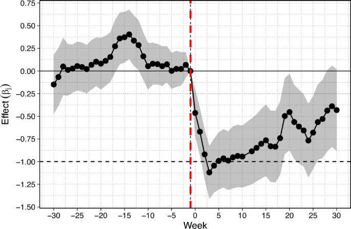
Event study: Retailer 2. Spanish Supermarket. Datamarket. This figure shows the estimates of the degree of VAT pass-through. Each coefficient bandwidth represents the 95% confidence interval. The vertical red and dashed line (-.-.-) represents the last week before the VAT cut (Week -1), which is the time period that we take as a reference. Sources: Authors’ calculations based on Datamarket
Additional tables
See Table 4.
Product classification
Given the broad coverage of products sold by each retailer, we also need to identify and assign a COICOP code to each product, and we obtain the brands using natural language processing techniques.
5.1 Data sources
In addition to prices, both Datamarket and DPD Prisma datasets contain text information. These two data sources contain the name and description of each product being sold (e.g., “sliced bread 500 gr.”), and the section or location of the supermarket where it is sold (following the example above: “breads, bakery”). We concatenate these two dimensions into a single piece of text. This resulting text for each product is hereinafter referred to as the product description. The product description also includes other information, such as the weight of the product (for example, 1 kg, 1l, 250g) or the brand name. We do not perform any kind of pre-processing steps for the product descriptions since, as we will mention later, we will rely on novel tokenizers that are able to detect all kind of characters within the text.Footnote24 One advantage of using web-scraped product description data is that this piece of text associated to each product is a short sentence (for example, “3 x frozen margherita Pizza extra cheese, Frozen food / Prepared dishes / Pizzas”). Usually, when performing a text analysis in economics, it is preferable to use short sentences in the modeling phase instead of large chunks of text (Hansen and Ash (2023)). However, the short text may contain some noise that can confuse the trained classifier. Following the previous example, the word “cheese” may suggest that this product description should be assigned to the COICOP category “Cheese”. This is one of the reasons why we choose to perform an algorithmic supervised classification task over a dictionary-based strategy. Using labels in order to minimize some loss function in the training phase reduces this kind of noise-related lower model accuracy. Besides, not only would a dictionary-based perform worse; also, it would be very time-consuming to keep on updating the dictionary terms for every product entry and exit from the market.
5.2 Data labeling
For the data-labeling phase, a pre-trained Sentence Transformer (Reimers and Gurevych) is used to encode product descriptions. A Sentence Transformer is a natural language processing (NLP) model designed to convert sentences or phrases into numerical vectors in a high-dimensional space. These vectors capture the semantic meaning of sentences, enabling tasks such as similarity search, which is our case. By converting sentences into numerical vectors, similarity can be calculated between them using distance measures. This kind of models do not use tokenized text; i.e., sentences (product descriptions) are encoded within the Transformer with no prior pre-processing or text cleaning. String punctuations, stop-words, and other types of language nuances are not removed from the text. The reason is that these Transformer models have their own tokenizer model as a pre-processing step and it is not required to preprocess the data before encoding sentences. This allows our information retrieval task to be more precise when executing the search. Then, once the produce descriptions are encoded (i.e., text is converted into a vector), a semantic similarity search using cosine similarity is conducted. This sequence of steps can be summarized as the following:
1. Suppose that we encoded all product descriptions within the Transformer. We now have a matrix of embedding NxL, where N is the total number of product descriptions and L is the maximum sequence length allowed by the transformer; that is, the maximum number of tokensFootnote25 that the Transformer can transform into a vector. We set the maximum length to 128 tokens. This embedding matrix can be seen as a “similarity” matrix.
2. Suppose we want to find products that are semantically similar to “3 × frozen margherita Pizza extra cheese, Frozen food / Prepared dishes / Pizzas”. We look for the encoded product description and measure the cosine similarity between the product description and all remaining product descriptions. Cosine similarity is calculated as:
where x and y are row vectors (x may be our product description). Euclidean (L2) normalization projects the vectors onto the unit sphere, and their dot product is then the cosine of the angle between the points denoted by the vectors.
3. Once we have the 1xN cosine similarities vector, we can sort that vector and yield the top K similar products to our “3 × frozen margherita Pizza extra cheese, Frozen food / Prepared dishes / Pizzas” product description.
We assign a Coicop 5 to each product description at once to the retrieved list after having manually reviewed each item. This allows us to rapidly label multiple similar product descriptions. A more detailed snapshot of how this task is performed can be seen in Fig. 20. This process is repeated until a sufficient number of manually tagged samples per Coicop 5 category are obtained.

Manual Bulk Labeling of similar products to ‘Pasta ‘. We used the Argilla user interface and API https://github.com/argilla-io/argilla
The data set used for labeling purposes consisted of approximately 54000 Spanish product descriptions, resulting in a labeled sample of around 10% of product descriptions on average for both countries, as can be seen in Table 6.
5.3 Methods
5.3.1 Model architecture
As Hansen et al. (2023) mention, the Natural Language Processing field has been substantially transformed in the last few years. Vaswani et al. (2023) proposed a new framework (called self-attention) that enables a neural network to weigh the importance of different elements in an input sequence and dynamically adjust their influence on the output. This is especially important for language processing tasks, where the meaning of a word can change depending on its context within a sentence or document. In our case, the interaction of certain key words determines COICOP categories. For instance, “3 x frozen margherita Pizza extra cheese, Frozen food / Prepared dishes / Pizzas” should be assigned a COICOP of ”Pizzas and quiches”. Some words, such as “cheese”, may be interacting with its surrounding words (such as “pizza” or “extra”) to indicate that it is indeed a “pizza”. This kind of interaction is what new natural language processing models are capable of capturing. In fact, in our paper, we use a model governed by the self-attention mechanism.Footnote26
Following Hansen et al. (2023), we use a DistilBERT (Sanh et al. (2020)) model to first domain-adapt it to our product description dataset and later to train it with the labeled subsample. A DistilBERT model is a smaller, distilled version of BERT (Devlin et al. (2019)). It is created through a process called knowledge distillation, where a larger, more complex model (in this case, BERT) is used to train a smaller model with similar capabilities. The objective is to transfer the knowledge from the larger model to the smaller one while reducing its size and computational requirements. DistilBERT aims to retain as much of BERT’s performance as possible while being more efficient in terms of memory and inference speed. Moreover, we choose a multilingual DistilBERT model; that is, as it name says, it can handle multiple languages. These models learn to encode and understand the context and meaning of words in multiple languages by capturing the relationships and patterns within the text during the training phase. By doing so, they acquire a cross-lingual understanding that allows them to transfer knowledge from one language to another. This means that the model can generalize its understanding of languages across different languages, even if it has not been explicitly trained on a specific language.
5.3.2 Domain adaption
We domain-adapt a pre-trained model with our product description data. Domain adaptation of a pre-trained model involves adjusting a model that has been trained on one type of data to work well on a different type of data. In machine learning, each type of data is called a domain, and the pre-trained model is trained on a specific domain called the source domain. However, when we want the model to work on a different domain called the target domain (product description data), we need to adapt it. Adapting the pre-trained model is necessary because the target domain may have some differences compared to the source domain. These differences could be due to variations in how the data was collected, differences in the data represents, or changes in the characteristics of the data itself. In essence, the main idea behind domain adaptation is to make the pre-trained model able to handle the differences between the source and target domains. This is done by adjusting the model so that it can transfer its learned knowledge effectively to the target domain. More specifically, this is done by removing randomly selected words from the product description data. Once words are deleted, the model updates its parameters by predicting the deleted words. We perform this task for the whole sample of product descriptionb data shown in Table 6. For this purpose, we use a DistilBERT multilingual model (Sanh et al. (2020)) pre-trainedFootnote27 on multiple languages and domain-adapt it to our product description data. We use the cased version since we do not perform ay kind of pre-processing within our product description data. Note that this could be easily extended as well to other languages, such as French, German, etc.
5.3.3 Training
There is scarce literature on what methodology should one follow to classify food products into official statistics’s categories. To our knowledge, there is only one paper relating this kind of problem. Lehmann et al. (2020) proposed using a transfer learning with a convolutional neural network trained on German human labeled data to infer and predict for French product description data. Once we have the multilingual DistilBERT model adapted to our data, we perform cross-validation over a hyperparameter space using our Spanish labeled subsample. The model we use is the same domain-adapted DistilBERT multilingual model from the previous step. We split our labeled subsample into a 70% train and 30% test sets to perform cross-validation over the training set. The hyperparameter space can be seen in Table 7.
For model evaluation, we monitor the average F1-score over the 3-folds. We select the model with highest average F1-score. Once we found the best hyperparameters,Footnote28 we fit the model on the whole training subsample and infer for the test set sample and check the model performance over all E-COICOP labels.Footnote29
5.3.4 Model comparison
To prove that our methodology is sufficiently accurate, we compare our model with another set of models. More specifically, we choose train and validate within the same test set of the previous step, the following models:
Gradient Boosting Classifier: a gradient boosting classifier is a machine-learning algorithm used for supervised learning tasks, particularly for classification problems. It belongs to the family of ensemble methods, which combine multiple weaker models (often referred to as base learners) to create a stronger predictive model. The main difference between this model and and our chosen model is that this model isn’t able to scale for other non Spanish product description data.
Moreover, some data pre-processing must be done in order to train and test for this model. In fact, we tokenize the text, deleting stopwords and removing string punctuation’s, lemmatize each word and create the term-frequency matrix. This matrix constitutes the input of this model. Then, we perform again cross-validation over a hyperparameter space that can be seen in Table 8. We fit the train with the best set of hyperparametersFootnote30 with the training set and evaluate for the test set. Note that, for model comparison, both training and test sets must be the same for all models.
SetFit (Tunstall et al.): this algorithm takes advantage of Sentence Transformers’ (Reimers and Gurevych) ability to generate dense embeddings based on paired sentences. In the initial fine-tuning phase stage, it makes use of the limited labeled input data by contrastive training, where positive and negative pairs are created by in-class and out-class selection. The Sentence Transformer model then trains on these pairs (or triplets) and generates dense vectors per example. In the second step, the classification head trains on the encoded embeddings with their respective class labels. At inference time, the unseen example passes through the fine-tuned Sentence Transformer, generating an embedding that when fed to the classification head outputs a class label prediction. A nice advantage of this model it can be trained using a multilingual pre-trained model. In fact, we train this algorithm using the same domain-adapted, multilingual model for the training process with 15 iterations, 5e-5 as learning rate and a batch size of 16. We then infer for the test set to allow model comparison.
5.4 Results
Looking at Table 9, we observe that our model outperforms the other selected algorithms. We present several evaluation metrics for the 30% test set of our labeled dataset. First, the precision measures how many of the positive predictions made by the model are actually correct. It can be seen that our model predicts 95% of the cases correctly. Second, the recall quantifies how well the model captures all positive instances in the data set.
A high recall value indicates that the model effectively identifies a large proportion of positive instances correctly, minimizing the number of false negatives. A low recall value suggests that the model misses a significant number of positive instances, resulting in a high rate of false negatives. However, our model outperforms the others in terms of recall. Finally, the F1-score, measured as the harmonic mean between precision and recall, is also 95%. This means that the model has a low rate of false positives (high precision) while effectively capturing most of the positive instances (high recall). It is noteworthy that the SetFit algorithm, designed to perform well with few labels per category, underperforms our chosen method, even if this algorithm also supports a multilingual setup. To our knowledge, this is the first attempt within economics research in comparing an easy-to-implement few-shot classification method with other state-of-the-art natural language processing models. A detailed table with all precision, recall, and F1-score metrics can be seen in Table 10.
About this article
Cite this article
Forteza, N., Prades, E. & Roca, M. Analyzing VAT pass-through in Spain using web-scraped supermarket data and machine learning. SERIEs (2025). https://doi.org/10.1007/s13209-025-00309-w
- Received
- Accepted
- Published
- DOI https://doi.org/10.1007/s13209-025-00309-w
Keywords
- VAT pass-through
- Price rigidity
- Inflation
- Consumer prices
- Heterogeneity
- Microdata
- Web-scraped data
- Machine-learning
JEL Classification
- E31
- H22
- H25