Recent searches nowadays discuss the technology for 5G and 6G of OWC systems. Several advantages characterize OWC as high bandwidth, security and capacity, and low interference and crosstalk (Aly et al. 2023). Also, OWC is characterized by utilization in both illumination and communication systems but suffers from coverage performance limitation due to using LED (Ding et al. 2016, 2022). In order to increase the system data rate, recent searches focused on multiple users and transmitters (Kadan and Haliloğlu 2023). To improve the system capacity, several searches used various MIMO techniques in OWC (Fath and Haas 2012; Ma et al. 2017).

Nelson et al. used non-Lambertian light beams in MIMO-OWC, and the same data is sent to all transmitters based on the enhancement in LED fabrication utilizing the solid-state (Nelson et al. 2024; Hande et al. 2023). The author in Moreno (2006) decreased the complexity utilizing spatial distribution of LED radiation. Deep ultraviolet LEDs (Zhou et al. 2024) in conjunction with a high power AlGaN‐based ultrathin tunneling junction produces distinct non-Lambertian light beams (Shi et al. 2020; Song et al. 2020).

Strinati et al. used a Single Input Single Output (SISO) channel in OWC with non-Lambertian light beams (Strinati et al. 2019), where asymmetrical emission of one optical beam is used to focus more optical power on the user (Faini et al. 2023). While Y.Zhang et al. utilized Monte-Carlo based on non-Lambertian pattern radiation for the OWC source (Zhang et al. 2023). G. Dawei et al. proposed an Extreme Learning Machine (ELM) based receiver to jointly handle the LED nonlinearity and cross-LED interference (Dawei and Qinghua 2019). Additionally, Gao et al. created a data-aided receiver in which data is employed as a virtual training sequence in ELM training and suggested ELM-based noniterative and iterative receivers to efficiently handle LED nonlinearity and memory effects (Gao et al. 2020).

These days, scientists are trying to find widespread uses for the benefits of ML and Deep Learning (DL) solutions in the business, scientific, engineering, health, and economic sectors. ML, which uses data and algorithms to mimic how humans learn to achieve increased accuracy, is regarded as a crucial area of Artificial Intelligence (AI) and computer science.

The main problem associated with MIMO-OFDM VLC is that its signal exhibits high peak-to-average power ratio (PAPR), which causes nonlinear distortion and consequently performance degradation. There are different methods to reduce PAPR while the ML used in PAPR reduction and outperforms other PAPR reduction techniques. Our proposal in this work uses ML to improve the performance of the system and the reduce the nonlinear distortion due to PAPR (Da Silva 2024). Utilizing OFDM in the MIMO VLC system makes cancellation to inter-carrier interference (ICI) and inter-symbol interference (ISI) due to utilizing the orthogonality and cyclic prefix (Kumar and Pandey 2009).

Object detection has significant research implications in computer vision, making it applicable to a wide range of applications. The core of object detection is the need to classify a specific object category and the requirement to use bounding boxes to determine location information. Given how crucial feature extraction is, one of the major turning points in object detection in recent years is the adoption of deep Convolutional Neural Networks (CNNs).

CNN-based object detectors can be divided into two categories, one-stage detectors such as Faster Region-based Convolutional Neural Networks (R-CNN) with breaking through the limitations (Zhu et al. 2021)

In Zhong et al. (2019), authors improved localization accuracy utilizing Loc-Net for faster R-CNN and region-based Fully Convolutional Networks, or R-FCNs (Liu et al. 2023; Su et al. 2024; Xie et al. 2018) improved spatial pyramid matching for scene recognition while (Jiang et al. 2024) analyzed the network robustness based on CNN and Spatial Pyramid Pooling (SPP) Net (Xiong et al. 2023), and two-stage detectors, such as SSD (Qian et al. 2023; Ni et al. 2023).

Several feature fusion strategies, including image pyramids, FPN, DSSD, and FSSD (Wang et al. 2023; Li et al. 2023) have been proposed to address the issue of scale variation. One of SSD primary benefits is that it uses an approach that combines various scale features to enhance detection performance. In a traditional SSD, information about small objects can only be extracted from one layer.

In ML, AdaBoost, is a boosting ensemble technique. It is predicated on the idea that students grow in steps. Every learner after the first is updated based on his previously mature learner, except the first. Additionally, each instance with erroneously classified instances receives a new assignment of weights with higher weights. Apart from its speed, simplicity, and ease of programming, AdaBoost stands out for its ability to be combined with any ML algorithm. Nevertheless, it has a high sensitivity to noisy data. Yan et al. (2023) proposed an anchor-free framework. Combining various scale features to create more useful feature maps using the skip connection and hyper-column approaches that were proposed by Omar and Abd El-Hafeez (2024).

In this paper, we propose a MIMO-OWC system with the non-Lambertian light beam in typical indoor scenarios and the estimation of the performance depends on the effect of the Access Point (AP) spacing with actual LED beams. Based on the results in Ding et al. (2018), the main contributions of this paper are decreasing the SNR’s CDF and enhancing system performance. Moreover, the work in this paper applies the non-Lambertian light pillars specifically and the cost-effective LEDs to arrange MIMO-OWC joins in the typical indoor environment. Both homogeneous and heterogeneous non-Lambertian MIMO arrangements are investigated. We used a low-intricacy RC MIMO calculation to evaluate the spatial convergence execution. As reported in Zhang et al. (2016), RC is considered to be optimal in the sense of error performance for an intensity modulated direct detection multi–input–multi–output optical wireless communication (IM/DD MIMO-OWC) over log-normal fading channels, where the authors proved that the optimality of RC under a much weaker condition in the sense of maximizing both large-scale and small-scale diversity gains for any space signaling.

In that context, to extract enough features, an effective feature fusion module that embeds freshly designed modules is incorporated into the MF-SSD. The Two-branch Residual Dilated Convolution Module (TRDCM) and the Two-branch TRDCM used in this framework are designed using dilated convolution with various dilation ratios. The TRDCM increases the receptive field without incurring additional computing expenses. To demonstrate the effectiveness of our suggested detector, we performed experiments on SNR and CDF of SNR datasets. Another strategy is based on applying the integration between SSD and the AdaBoost ML mode to compare the two models and choose the best model for decreasing the Signal-to-Noise Ratio (SNR) and Cumulative Distribution Function (CDF).

The necessity to solve particular issues in MIMO-OWC systems, like dynamic noise, interference, and precise CDF prediction under changing SNR conditions, is what spurred the integration of MF-SSD with AdaBoost. AdaBoost offers robust regression by iteratively improving predictions and giving harder-to-predict samples greater weights, while MF-SSD uses multi-path feature fusion to maintain spatial resolution and capture multi-scale information (Chowdhury et al. 2020). Compared to solo DL models and conventional ML techniques like SVM or random forests, this combination improves prediction accuracy and robustness to noisy data. The suggested method, which is backed by theoretical analysis and quantitative comparisons that demonstrate its resilience and efficiency, raises the bar by enhancing connection reliability, throughput, and scalability in OWC scenarios.

To overcome the limitations in the introduced framework, the influence of noisy samples is reduced during training by using loss functions. Additionally, to lower computational expenses, use backbones like the DenseNet121 model. In order to capture dynamic changes in the MIMO-OWC environment, the model should also incorporate multi path feature fusion.

The following lines summarize the main objectives:

• Collecting the datasets of the results in Ding et al. (2022) where the SNR and CDF shape is the basis of the dataset used in the proposed models.
• A new framework for signal detection, called MF-SSD, is applied to address multiscale issues, particularly when there are numerous channel variations.
• We have developed a new effective feature fusion module that can extract enough signal features of different kinds to enhance performance for CDF of SNR prediction values.
• The TRDCM and TRDACM are two newly designed modules included in the proposed feature fusion module to enhance contextual information with sufficient features through these two modules, and hence decrease the CDF values.
• In addition, another model is introduced based on the integration between the SSD and AdaBoost models to determine which model performs better than the other.
• Furthermore, K-fold cross validation is utilized to evaluate the system performance and overcome the over- fitting.

This is how the rest of the paper is organized. In Sect. 2, the system model is explained. In Sect. 3, the dataset extraction process is described. Section 4 displays and discusses the obtained results. Section 5 is devoted to the main conclusions.

The proposed indoor system model is illustrated in Fig. 1. MIMO-OWC is studied in a room with dimensions 5, 5, and 3 m at the height of the receiver plane 0.85 m. There is a different radiation pattern as shown in Fig. 2 where 3D pattern radiation is considered: (a) traditional Lambertian light beam, (b) LUXEON Rebel light beam, and (c) NSPW345CS light beam (Moreno 2006).

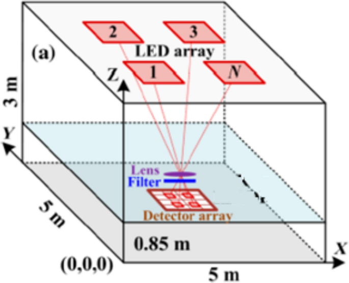
Indoor system model

Full size image

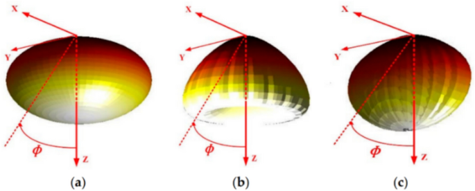
3D spatial radiation pattern from a typical view of a traditional Lambertian light beam, b LUXEON Rebel light beam, and c NSPW345CS light beam (Moreno 2006)

Full size image

To analyze the performance of the MIMO-OWC system, the LED light source follows the traditional Lambertian pattern as shown in Fig. 2a, where the radiation intensity can be calculated (Ding et al. 2019)

where  is the irradiance angle,  represents the Lambertian order and its equation is

 is the half-power angle of the Lambertian beam.

Our OWC system has a channel gain containing both of Line of Sight (LoS) and Non-Line of Sight (NLoS) components. The power of NLoS is very small, thus, NLoS is ignored and only the LoS is considered. The channel gain of LoS for known the Lambertian is calculated as (Ding et al. 2016)

where  is the physical area of a photodetector,  is the distance between the n^th transmitter and the m^th receiver,  is the optical concentrator gain,  is the irradiance angle from the n^th transmitter to the m^th receiver,  is the incidence angle from the n^th transmitter to the m^th receiver,  is the field of view (FoV) at the receiver.

The optical concentrator gain is given by Ding et al. (2016):

where  is an internal refractive index at the receiver.

The channel gain for the second case in Fig. 2b is the LUXEON Rebel beam case which is calculated by Ding et al. (2016)

The channel gain for the third case in Fig. 2c is the NSPW345CS case, which is calculated by Ding et al. (2016)

where  is the azimuth angle of the mth receiver to the nth optical AP.

As shown in the system model of Fig. 1, four transmitters and one receiver with four photodiodes (PDs), the output optical signal of the receiver is calculated by Ma et al. (2017) and Nelson et al. (2024)

where x = [x₁, x₂, x₃, x₄] are emitted transmitter symbols, y = [y₁, y₂, y₃, y₄] are the received symbols at the receiver, n = [n₁, n₂, n₃, n₄] are the additive white Gaussian noise (AWGN) values at the receivers.

One can consider case 1 for the known Lambertian beam for the MIMO-OWC system, where the channel gain matrix, H, is given by:

Similarly, the channel gain matrix for cases 2 and 3 is given, respectively, by

Harald Hass (Fath and Haas 2012) calculated SNR for MIMO-OWC by applying the same repetition coding with low complexity

where r is the responsivity of the PDs,  is the emitted power of all transmitters, N₀, N_t, and N_r are noise power, number of APs, and number of PDs, respectively.

To construct the configuration of the non-Lambertian, the MIMO-OWC system with distributed transmitters Aps has two LEDs of Lambertian pattern and two LEDs of NSPW345CS non-Lambertian light beams. Firstly, for the inter-AP heterogeneous light beam configuration, the NSPW345CS non-Lambertian light beams are utilized to replace a part of the Lambertian homogeneous configuration and the channel gain can be calculated by Ding et al. (2016)

Secondly, for the intra-AP heterogeneous light beams configuration, the NSPW345CS non-Lambertian light beam is added to each AP of the above Lambertian homogeneous configuration; we can calculate the MIMO channel gain matrix H to be as Ding et al. (2016)

The main parameters of configuration for the system model are shown in Table 1.

We consider the indoor MIMO-OWC system with 4 APs in the ceiling, where two LEDs have a Lambertian pattern, and two LEDs have an NSPW345CS pattern to get the overall configuration with the non-Lambertian pattern. The proposed models use the results from Ding et al. (2022) as datasets to be imported into the proposed models.

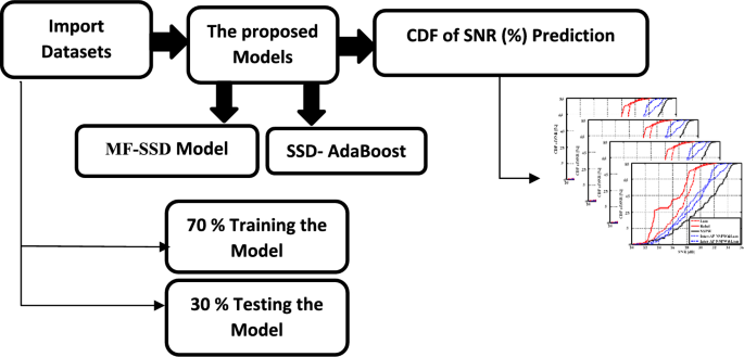
Two models are proposed in this paper. The first one is MF-SSD, which predicts the CDF based on SNR by utilizing DenseNet121 as its backbone. The second boosts the system performance by integrating the SSD with the AdaBoost ML model. Furthermore, the K-fold cross validation technique is employed the judge the system efficiency instead of applying the validation technique for the dataset. The block diagram of the introduced framework is introduced in Fig. 3.

Block diagram of the introduced framework

Full size image

Figure 3 illustrates the steps of the proposed system; start with importing the datasets into the proposed models (MF-SSD and SSD-AdaBoost). The results from the models are figured into the relation between CDF and SNR for each model. The datasets are divided into 70% training data, while the 30% left data is used to test the model.

3.1 Dataset

The MF-SSD and SSD-AdaBoost DL models are trained using the datasets used in this investigation, which were extracted by Ding et al. (2022). These datasets provide crucial statistics for OWC scenarios as shown in system model. A comprehensive dataset is used to train and evaluate the suggested models, comprising 155 vectors of transmitted signals propagated through an indoor channel. The dataset is divided into 70% training and 30% testing and validation 5% validation and 15% testing) in order to train the DL models. The datasets SNR and CDF shapes are used to optimize the models during the training stage. The models are operated in two stages. The SNR and its CDF distribution of SNR are used to train the model online. Next, testing is conducted to predict the CDF distribution as output by using the SNR as input. The model gains knowledge of the channel properties that will be used in testing during the training phase. Therefore, the system performance is enhanced through a reduction in the cumulative distribution. The proposed dataset is analyzed based on the OriginPro program to be imported into the Python software as shown in Fig. 4.

Samples of the proposed dataset transformation into a 2-D image

Full size image

In order to overcome this issue, the K-fold cross-validation technique is used to evaluate the model robustness across various dataset subsets and make sure it functions well in a range of scenarios. Furthermore, by allowing the model to more effectively capture and generalize intricate patterns in SNR and CDF distributions, multi-path feature fusion is used to assist get around the dataset restrictions. Even if the dataset does not explicitly cover every case, this fusion enables the model to learn richer representations, increasing its resilience to dataset fluctuations. Dilated convolution layers, which record contextual information at various scales, are incorporated into the fusion module of multipath fusion. By doing this, the model is able to ignore noise and recognize important features. By emphasizing pertinent features, the feature fusion technique lessens the effect of noisy features. Last but not least, the suggested framework captures contextual and hierarchical patterns, improves generalization by combining shallow and deep features, and allows adaptation to situations that are not visible by reducing the influence of noisy data through multi-scale context learning. It picks up characteristics of MIMO-OWC systems that are resistant to environmental fluctuations.

The receptive field can grow exponentially with dilated convolutions without requiring more parameters or sacrificing resolution. Several scale-contextual information from various spatial resolutions is captured by employing several dilation rates in the Two-Branch Residual Dilated Convolution Module (TRDCM) and TRDACM modules, notably dilation rates of 2, 3, and 5. The goal of lower dilation rates of 2 is to recover boundary information and fine-grained features. The model can include long-range relationships and a wider semantic context when the dilation rates are higher (3 and 5). This combination aids in the model’s integration of local and global information, which is essential for precisely forecasting SNR-CDF pairings in MIMO-OWC systems with a range of channel circumstances. Especially in settings where signal quality varies, its multi-scale receptive field architecture increases detection accuracy and resistance to noise.

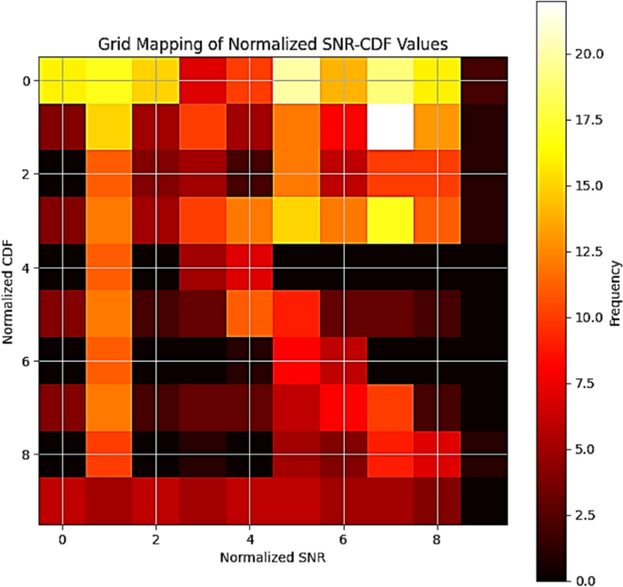
The heat map that illustrates a grid mapping of normalized SNR-CDF values and shows the correlation between normalized SNR and normalized CDF is explained in Fig. 4. The figure shows a discretized grid of SNR (horizontal axis) and CDF (vertical axis), with associated frequencies represented by color intensity, according to the grid mapping of normalized SNR-CDF values. The probability that a random variable (SNR) takes a value below or equal to a specific threshold is measured using the CDF. The CDF values are scaled to a constant range (0–10) due to normalization. Dark hues (black, red) indicate low frequencies (fewer occurrences), whereas the color bar on the right shows the frequency of occurrences for particular combinations of normalized SNR and CDF values. On the other hand, high frequencies (more occurrences) are represented by bright hues like white and yellow. The color bar indicates that the maximum frequency is 20. A high frequency is seen around SNR = 5–7 and CDF = 4–6, indicating that these SNR-CDF pairs predominate in the sample. Sparse occurrences occur near SNR = 0–2 and CDF = 8–9.

Through the grid-based mapping of the normalized SNR and CDF values, a particular combination of SNR and CDF is represented by each cell in this grid. Next, a small object in the grid is mapped to each SNR-CDF pair; this process is known as creating the labels. In more detail, the anchor boxes must be conceptually modified to meet the requirements of the task at hand. Anchor boxes are used in place of bounding boxes in a 2D image space to adjust SNR and CDF prediction. Upon examination of the data distribution and range, it is noted that the proposed model is characterized by an SNR range that spans from a minimum of − 2.68 dB to a maximum of 135.72 dB and a CDF range that oscillates between a minimum of 11.60 and a maximum of 35.47. As a result, low CDF and SNR values are covered by the small scale, which ranges from 15 to 30, mid-range values are covered by the medium scale, which ranges from 30 to 75 dB, and high SNR and CDF values are covered by the large scale, which ranges from 75 to 135 with aspect ratios that depend on the distribution of SNR versus CDF, which is 1:1, 1:2, or 2:1.

3.2 Single shot detector DL model

The SSD algorithm enables object localization and classification to be completed in a single neural network forward pass (Fath and Haas 2012). It is claimed that the SSD algorithm is faster and easier to train and faster. There is a noticeable speed boost from the removal of region proposals and the feature resampling step.

In this paper, the SSD architecture is modified to use the pre-trained DenseNet121 as a backbone to extract the signal features and enhance the framework performance. In addition, the introduced framework is performed for CDF prediction based on SNR. The dataset is reshaped to be in a 2-D tensor in the form of a feature map for the input. To process the features that are taken out of the base network, more layers are added. Convolutional layers with 2 × 2 Kernel, pooling layers, and activation functions are designed to enhance the execution. Lastly, the prediction layers have continuous values that show the anticipated SNR and CDF. Fully connected layers that produce the CDF for specified SNR inputs are used to accomplish this.

In this work, the DenseNet121 model serves as the feature extractor. The SSD detection layers are changed so that continuous CDF values rather than bounding boxes are predicted. Additionally, swap out the SSD classification and localization heads for a single regression head that can make direct CDF predictions. The proposed modified architecture in DesnNet12 is explained in Table 2.

• First Convolutional Layer: 1024 input channels (this input is derived from the feature map of the DenseNet121 backbone). Moreover, 256 output channels, a reduction in the feature map depth. Kernel size of 1 × 1 (pointwise convolution decreases the feature map dimensionality without changing its spatial dimensions). This layer preserves the spatial resolution of the feature map by decreasing its depth (number of channels).
• Second Convolutional Layer: 256 input channels are compromised (from the layer above). Moreover, 512 output channels add depth to the feature map. Additionally, to capture more spatial context, a 3 × 3 kernel size is utilized. The spatial resolution decreases with a stride of two. Furthermore, a padding of 1 ensures that the output feature map is the same size as the input feature map prior to down-sampling. This layer down-samples the spatial resolution by a factor of 2, while increasing the number of channels to 512.
• Third Convolutional Layer: It consists of 512 channels for input and 128 output channels are used to lessen the feature map depth. Perform pointwise convolution to decrease the feature map’s depth by using a 1 × 1 Kernel size. To maintain manageability, this layer takes the feature map depth down.
• Fourth Convolutional Layer: It is employed to increase the number of channels and decrease the spatial resolution. The model has a stride 2 and 3 × 3 kernel and employs 128 input and 256 output channels. This enhances prediction performance by enabling the model to extract higher-level features.
• Fifth Convolutional Layer: Finally, it reduces the out channel again to 128 and point-wise convolutional with 1 × 1 Kernel.

3.3 Multi-path feature fusion single shot multi-box detector (MF-SSD) model

In this paper, several steps are introduced to enhance the system performance and decrease the CDF of SNR. The first step is preparing the dataset by normalizing the SNR and CDF of the SNR dataset. Next, features at different levels are extracted using the DenseNet121 model. This work implements two dilated convolution-based modules that fuse the deep and shallow features of the feature fusion module. The MF is the process of combining the fused features over several pathways. To estimate the CDF given the SNR, the prediction head layers are finally applied to the final fused feature map.

The SSD model, in this work, is modified to be composed of the number of channels in the input feature map for this convolutional layer which is 1024. There is a total of 16 channels total because the output feature map has 4 × 4 channels. For every default box, each channel translates to the prediction of four bounding box coordinates. To preserve the spatial dimensions of the input feature map, a padding of 1 is added to the convolutional Kernel, which has a size of 3 × 3. The bounding box locations are predicted by this layer. Each cell has four default boxes, and each box prediction has four coordinates. To train the MF-SSD, two steps are needed. For the top 28 layers, the required grad setting to false in the first step, freeze train is adjusted. Furthermore, the required grad setting for every layer in the second step, the unfreeze train is neglected. Using the Adam optimizer, the freeze train’s batch size, learning rate, and weight decay to 32, 0.00035, and 0.00035, respectively are utilized. To unfreeze the train and set the batch size, learning rate, and weight decay to 16, 0.00011, and 0.00045, respectively, we also used the Adam optimizer. Both the freeze train and the unfreeze train have been conducted using a learning scheduler with a step size of 1 and a gamma of 0.94. The total epochs are set to 350 for the unfreeze and freeze trains.

The MF-SSD architecture is previously shown in Fig. 4. The FFM is first presented, along with the Connection Module (CM), which are rectangular boxes that are blue and green. The orange rectangular boxes represent the TRDCM, and the purple rectangular boxes represent the TRDACM.

3.3.1 Connection module (CM)

One lower-level feature map and one higher-level feature map make up the CM. A 1 × 1 convolution is used in our framework to match the channel numbers of both inputs. Next, feature maps at higher levels are up-sampled to match the lower-level feature map’s size, even though they usually have lower resolution. This up-sampling employs bilinear interpolation since experiments have shown it to be more effective than deconvolution. Additionally, a concatenation approach is used to fuse the feature maps, combining them along the channel dimension without enlarging their spatial size as explained in Fig. 4.

3.3.2 Two-branch residual dilated convolution module (TRDCM)

As seen in Fig. 4, through the preservation and utilization of high-resolution features from deeper layers, the TRDCM seeks to improve feature detection for our 2-D grided images. Dilated convolutions are used to increase the receptive field without adding more computational cost by sampling at different locations. The TRDCM improves the semantic information available for minute changes in the channel by fusing features from shallower layers (like the first convolutional layer) with deeper layers. 1 × 1, 3 × 3 (dilated ratio 2), and 3 × 3 (dilated ratio 3) convolutions are found in the first branch. On the other hand, 1 × 1, 3 × 3 (dilated ratio 3), and 3 × 3 (dilated ratio 5) convolutions are used in the second branch.

3.3.3 Two-branch residual dilated add convolution module (TRDACM)

To improve the contextual information and solve problems like gradient vanishing and limited receptive field, the TRDACM is presented as shown in Fig. 5. To adjust the channel numbers, a 1 × 1 convolution is performed first. Next, to extract contextual information, both branches employ 3 × 3 dilated convolutions with various dilated ratios. Dilated ratios of two and three are used in the first branch and three in the second. Additionally, for improved optimization, include residual connections without further convolution. A concatenation attention approach is used to combine the outputs of the two branches.

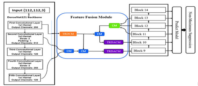
The architecture of MF-SSD

Full size image

3.4 Adaptive boost ML algorithm (AdaBoost)

In ML, an adaptive boost, or AdaBoost, is a boosting ensemble technique. It is predicated on the idea that learners develop in sequential order. Every learner after the first is updated based on his previously mature learner, except the first. Additionally, each instance with erroneously classified instances receives a new assignment of weights with higher weights. Apart from its speed, simplicity, and ease of programming, AdaBoost stands out for its ability to be combined with any ML algorithm. Its sensitivity to noisy data is high.

The initial CDF values which are predicted by the SSD feature extraction process are fed as inputs for an AdaBoost model. Then, by merging several weak learners, the AdaBoost model can improve these predictions and produce a more powerful prediction model.

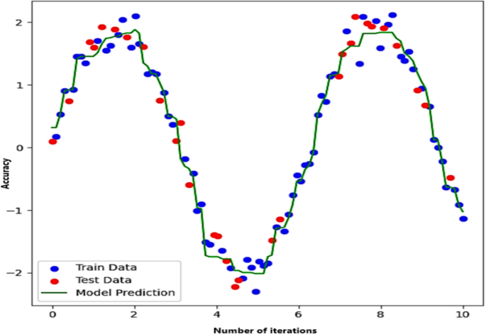
Figure 6 explains a plot with the number of iterations on the x-axis and accuracy on the y-axis. The independent variable, which appears to vary from 0 to about 10, is the number of iterations, indicating that the dataset was generated or sampled throughout a continuous domain. On the other hand, the dependent variable is accuracy. The numbers appear to fall between roughly − 2 and + 2, indicating that the data exhibits an oscillatory or periodic pattern. Additionally, the train data, points used to train the model, are represented by the blue dots. The oscillating pattern is closely followed by these dots. The test data, which are invisible data points used to assess the model’s performance, are represented by the red dots. The predictions produced by the model that was trained on the data are shown by the green line (Model Prediction). The line shows that the model has picked up on the underlying trend because it closely resembles the pattern of the train and test points.

AdaBoost ML model simulation parameters

Full size image

In Fig. 6, the AdaBoost selects decision trees to capture dataset variations. Additionally, 100 decision trees, or estimators, are employed. In other words, the AdaBoost model will fit 100 weak learners in a row, each of them attempting to fix the mistakes of the previous one. Stronger models are often the result of using more estimators, but overfitting risk and computational expense must be balanced. The learning rate in the framework is set to 0.1, which results in more gradual learning by regulating the amount of influence that each tree has on the final prediction.

3.5 SSD-AdaBoost model

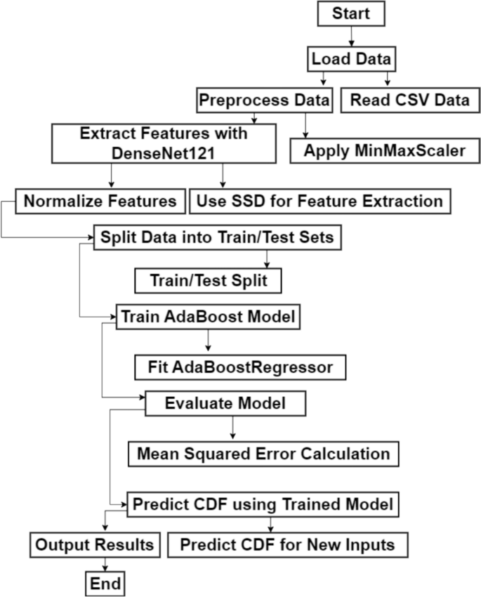
Based on the presented framework, five additional convolutional layers are added to the backbone (DenseNet121) in the SSD model. These layers preserve the spatial resolution of the feature map by decreasing its depth (number of channels) as mentioned in Sect. 3.3. Following feature extraction using the SSD and DensNet121 as the backbone, the CDF values are ready to be used as labels in the AdaBoost model. This method is applied in ML to boost the accuracy of predictions as seen in Fig. 6. Moreover, Fig. 7 demonstrates how the SSD model is applied to predict signal labels from a 2D grid of SNR and CDF data, by turning feature maps into insightful forecasts.

Flowchart of SSD-AdaBoost model

Full size image

Because it gives misclassified samples more weights during training, AdaBoost is known to be sensitive to noisy data and can increase the impact of outliers. In this paper, the AdaBoost weight threshold, which limits the maximum weight given to individual samples during boosting iterations to avoid overfitting to noisy data, is used to combat this problem. Additionally, utilizing strong learners like regularized decision trees rather than extremely sensitive ones like decision stumps. When dealing with noisy data, these trees perform better (Azadvar et al. 2021). Additionally, fusion with SSD emphasizes how AdaBoost focus on difficult samples is leveraged in conjunction with SSD feature extraction capabilities. In the domain of OWC systems, AdaBoost is preferred above other methods such as SVM or random forests. The iterative AdaBoost method dynamically modifies weights for misclassified data, which makes it appropriate for managing the ever-changing environmental conditions of OWC systems. The SSD models are also quite good at extracting spatial characteristics. The system may retain high-speed detection while concentrating on difficult areas (such as those with low SNR) when AdaBoost is included. AdaBoost is more appropriate for real-time OWC applications because it is computationally lightweight during inference, in contrast to random forest which does not have dynamic sample re-weighting or SVM which might be computationally costly for large datasets. When it comes to hard-to-classify samples, random forest is less adaptive. SVM is sensitive to Kernel parameter adjustment and computationally costly, although it works well for high-dimensional data.

Figure 7 shows the flowchart of a ML pipeline that combines DenseNet121, SSD, and AdaBoost regressor to forecast a dataset’s CDF. First, the dataset is loaded, which includes SNR and CDF values, among other variables. In order to optimize model performance by preventing some features from dominating others due to different scales, parse the dataset file, organize it for processing, and normalize the features to a consistent range ([0, 1]). The SSD is used to extract features further. Make that the SSD and DenseNet121 features are appropriately normalized (scaled). Lastly, divide the data into test and train sets. The model is trained using the training dataset, and its performance is assessed using the testing dataset. Lastly, the trained model may also anticipate new inputs and generalize to previously encountered data.

Figure 8 describes the correlation between normalized SNR and normalized CDF provided by the 2-D tensor. Various color intensities suggest the concentration of particular values in the dataset by indicating varying frequency levels. With the help of the input features (SNR), the SSD model is applied to this grid data to identify particular significant points of CDF of SNR. Ultimately, a sequence of object labels representing the output of the SSD model is shown, along with a class identifier designating the identified class. The location and size of the detected values are defined by the bounding box coordinates. Based on the input grid mapping, the output indicates that the SSD model has identified some CDF values with success.

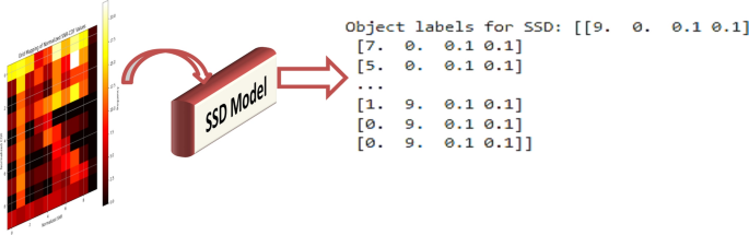
Sample of the SDD output based on SNR and CDF dataset

Full size image

Because of its special benefits in assessing system performance, especially in statistical and probabilistic analysis, the proposed model uses the Cumulative Distribution Function (CDF), which offers a thorough probabilistic description of the variable. When it comes to MIMO-OWC systems, CDF is very helpful in assessing the likelihood of reaching specific signal quality levels, providing information about system dependability under various circumstances. The cumulative probability distribution of different underlying performance measurements is naturally captured by CDF, allowing for indirect assessment of those metrics. By eliminating the need to explicitly track numerous measures, it streamlines the model and lowers computing complexity while maintaining a comprehensive view of performance. Ensuring dependable performance in a variety of environmental situations is one of the main design objectives for MIMO-OWC systems. The CDF is especially pertinent for evaluating system robustness since it directly represents the system capacity to sustain performance across a variety of SNR values. Our introduced framework is used to assess and maximize the possibility of reaching better system performance levels by concentrating on the CDF. Metrics such as SER and BER frequently offer point estimates of performance under particular circumstances, which may not accurately reflect how the system behaves in a variety of operating settings. A more sophisticated comprehension of system behavior in dynamic and unpredictable OWC situations is made possible by CDF, which, in contrast, captures the full distribution of performance. SNR frequently has a direct correlation with metrics like capacity and BER. CDF indirectly offers insights into these parameters without explicitly modeling them because it already captures the distribution of SNR values. This provides useful information about system performance without adding unnecessary repetition to the evaluation framework. Overfitting to several objectives is less likely when the model is trained and assessed using a single, cohesive metric, such as CDF. When used in real-world settings, this can enhance the model capacity for generalization.

In our proposed framework, there is no need for the validation set, because the DenseNet121 model serves as the foundation for feature extraction in the MF-SSD model in this paper. It is possible to make DenseNet121 model pre-trained weights, which are designed for generic feature extraction, non-trainable. These layers can be frozen to help concentrate training on task-specific elements such as the MF-SSD model higher-level layers and dilated convolutional modules. By examining the performance improvements, one can determine which components (like feature fusion modules) can be left untrainable and which ones require trainable parameters. The model feature fusion modules and semantic-rich layers appear to be optimized, as evidenced by its higher performance in both homogeneous and heterogeneous MIMO configurations. Layers for lower-level feature extraction might stay fixed. Finally, the need of a validation set in this improved OWC model can be lessened by utilizing the redundancy coding MIMO technique, the DenseNet121 backbone inherent strengths, and current performance indicators. The MF-SSD model performs better in every transmitter scenario by using newly developed modules and freezing pre-trained layers. In addition, the K- fold cross validation is added in this paper to evaluate the framework performance. This is done by dividing the training dataset into fivefold cross-validation rather than having a separate validation set, to evaluate the model on the remaining fold after training it on K − onefold. To evaluate performance, the folds and average the outcomes are rotated. In order to concentrate training on modules that enhance certain measures and freeze others, this paper adds important performance measurements such as accuracy, precision, sensitivity, and F1-score to evaluate the system efficiency. By preventing overfitting, these metrics guarantee that optimization efforts are in line with the task performance requirements as seen in Table 3.

As seen in Table 3, with an average accuracy of 98.73% ± 0.33, the MF-SSD model is very dependable when it comes to accurate prediction. The model is highly effective at detecting true predictions, which means it can effectively detect the presence of the condition it is designed to identify. Its average sensitivity is 98.25% ± 0.34. The model predicts a correct result with an average precision of 98.65% ± 0.35. Lastly, the model is robust in a variety of settings with an average F1-Score of 98.70% ± 0.27, which demonstrates a great balance between precision and recall. According to results shown in Table 3, both models function quite consistently throughout a range of K-fold values, which is essential for dependability in practical applications. Practically, the MF-SSD model performs marginally better than the SSD-AdaBoost model, but particularly in F1-Score and precision (Salama, et al. 2020), suggesting that it makes more accurate and well-rounded predictions. Both models standard deviations are low, indicating steady and reliable performance over the many folds.

As described in Sect. 3, the output of the two proposed models is shown about CDF versus SNR. In Fig. 9a the proposed model is the MF-SSD, where the SNR and CDF of the discussed homogeneous and heterogeneous MIMO optical wireless communication scenario is illustrated. Figure 9b shows the SNR cumulative distribution function with different heights of Aps.