Article Content
1 Introduction
Since the seminal work by Bendsøe and Kikuchi (1988), topology optimization has gained much popularity for the automatic design of structures. Among others, density and level-set based methods are some of the most popular approaches, see Sigmund and Maute (2013). Density-based methods optimize material distribution parameters volumetrically, whereas level-set methods optimize the shape of interfaces between predefined material phases. Both methods have advantages and drawbacks; the density-based method requires almost no prior knowledge of the final design; however, near-interface effects can be challenging to resolve, as boundaries are not explicitly defined. Level-set methods rely on a description of the interface between the phases and the shape of these interfaces evolves in the optimization process. Therefore, sensitivities are only present at the interface, which requires seeding inclusions of one phase into the other if the topology needs to change in 2D. In three-dimensional problems, inclusions can grow into the design from the design domain boundaries. However, this is not always sufficient to obtain satisfying topologies. Methods have been developed to seed new holes, as these are necessary for obtaining a more complex topology. Topological derivatives originated from the bubble method (Eschenauer et al. 1994) and were further expanded in the works by Sokołowski and Żochowski (1999), Burger et al. (2004), Allaire et al. (2005), Norato et al. (2007), and Sá et al. (2016). These methods evaluate the sensitivity of adding an inclusion at any given point and hence enable the optimizer to add inclusions where they are necessary.
Topology optimization for fluid problems was first introduced by Borrvall and Petersson (2003), who optimized the film thickness of Stokes flow between two parallel plates. Gersborg-Hansen et al. (2005) included the convective term in the governing equations and topology optimization has since been applied to a wide range of fluid problems, as described in the review of Alexandersen and Andreasen (2020). Density-based methods for fluids generally show good convergence toward solid–fluid designs. Evgrafov (2005) showed that the fluid power dissipation problem in Stokes flow is convex. When including the convective term, i.e., considering the Navier–Stokes equation, good designs are generally obtained when starting from a pure fluid initial design, such that there is fluid flow throughout the optimization domain. The importance of initial designs, which allow for fluid flow in the entirety of the optimization domain, is also highlighted in the study from Høghøj et al. (2020) in the context of topology optimization of two fluid heat exchangers. In density-based methods (and ersatz material level-set methods), the wall is not represented explicitly, which can be challenging when modeling near-wall effects and boundary conditions, as seen for conjugate heat transfer by Rogié and Andreasen (2023). Furthermore, the density-based approach allows pressure and fluid to leak through the solid regions, which are modeled as porous media. The issue renders interpolation choices very important, as discussed by Lundgaard et al. (2018) in the context of topology optimization for fluid–structure interactions.
Kreissl and Maute (2012) first studied flow topology optimization using the level-set method and solving the incompressible Navier–Stokes equation with the Heaviside enriched eXtended Finite Element Method (XFEM). Using a clearly defined boundary representation allows for the explicit treatment of the wall boundary conditions, for example, by Nitsche’s method whose accuracy can be controlled by a penalty parameter and mesh refinement. If the penalty parameter is insufficient, the boundary condition will be enforced poorly, such that fluid might slip or leak. Hence, it is important to set the penalty parameter adequately. However, opposite to the ersatz material method, no fluid flow is represented inside the solid domain.
Topology optimization for fluid applications using the level-set method and XFEM has since been extended to fluid–structure interactions, where Jenkins and Maute (2015) optimized the shape of external and internal boundaries of structures subject to fluid flow loading. Coffin and Maute (2016) used level-set methods to optimize structures subject to transient and steady-state natural convection. Villanueva and Maute (2017) demonstrated the use of ghost stabilization when using immersed methods in the context of both steady-state and transient fluid topology optimization. Most recently, Noël and Maute (2023) used level-set methods for the topology optimization of turbulent conjugate heat transfer problems, where the modeling of the flow, turbulence model, and heat transfer were realized using XFEM.
Level-set methods can also be used for topology optimization with other modeling approaches than XFEM. In the context of topology optimization of fluid systems, this has notably been done in the works of Feppon et al. (2019, 2021), where body-fitted meshes are generated at every design iteration, such that the velocity and pressure fields are always evaluated on a body-fitted mesh.
Irrespective of the analysis method, the initial seeding of solid inclusions in level-set based fluid topology optimization is a non-trivial task, as the final design often depends on the initial design. A similar influence of the initial seeding on the optimized design has also been observed in topology optimization of structures (van Dijk et al. 2013). For some combinations of physics and objective and constraint functions (e.g., linear elasticity and compliance minimization) in three dimensions, inclusions can grow into the domain from the sides, as observed by Aage et al. (2021). However, generally and more specifically in flow topology optimization, this is not necessarily the case.
In the context of compliance minimization, Barrera et al. (2020) proposed two approaches to seed holes in the material phase using a density-based method. To this end, the density field can spatially vary within the structural domain and is linked to the level-set field. In the optimization process, the density and level-set fields evolve simultaneously using design sensitivities. As the density approaches zero in a region, the linkage of density and level-set field is formulated such that the level-set field assumes a value associated with void. These methods allow for initializing the design domain with a uniform density without holes, as is common for density-based methods.
This work presents a method for density-based hole seeding in level-set topology optimization of fluid problems, extending the methods from Barrera et al. (2020) to flow problems. The fluid flow is modeled by Heaviside enriched XFEM which is similar to the method presented in Noël et al. (2022). The incompressible Navier–Stokes equation is stabilized using Pressure Stabilizing Petrov Galerkin (PSPG) and Streamline Upwind Petrov Galerkin (SUPG) stabilization schemes. Boundary conditions are imposed in weak form by Nitsche’s method (Nitsche 1971). Numerical instabilities due to small integration subdomains near the interface are alleviated by using face-oriented ghost stabilization, as described by Villanueva and Maute (2017). Density-based hole seeding is introduced by defining an explicit dependency between the density and level-set fields. To model the effect of a spatially varying density field on the flow, a Brinkman penalization term is introduced in the Navier–Stokes equation. This term needs to be accounted for in the formulation of the Nitsche penalization and ghost stabilization. The need for this is demonstrated by numerical studies. Topology optimization problems are solved with the hybrid density-level-set method bypassing the need for hole seeding in the initial design and prior knowledge about the final design. The optimization results obtained with the MORIS frameworkFootnote1 show that the proposed method eliminates the need for an initial hole-seeding heuristic.
The remainder of this paper is structured as follows: Sect. 2 presents the hybrid density-level-set parametrization; Sect. 3 the employed methodology for the fluid flow modeling; Sect. 4 the optimization formulation; Sect. 5 optimization results, and Sect. 6 concluding remarks.
2 Parametrization
In this study, two physical phases are assumed in the design domain, with being the solid phase and being the fluid phase. Their external boundaries are denoted by and , respectively, and the boundary between and is denoted . Figure 1 presents a schematic of the represented phases and their respective boundaries. The shaded color in symbolizes the presence of a spatially varying, relative density in the fluid phase.
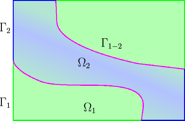
Design domain with two phases, and , as well as their interfaces to the exterior of the domain, and , respectively, and their common interface,
In the design domain, a level-set field, , with the threshold value is used to identify the phases and their common interface:
The parameterization allows for an explicit treatment of the boundaries of the distinct physical phases, both at the boundaries of the domain and on the interfaces between the two phases. The enforcement of boundary conditions is discussed in Sect. 3.2.
Within the fluid phase, , a relative density variable, , is deducted from the level-set value, , following the single field formulation of Barrera et al. (2020). is defined by:
where is the upper bound of the level-set field. The density variable, , is defined within the fluid phase and allows for a continuous transition from fluid to solid. The solid domain is omitted from the analysis of the fluid state.
The design representation is discretized on regular quad (2D) or hexahedral (3D) meshes. These meshes can be hierarchically refined and support B-spline discretization. This work adopts the discretization strategy of Noël et al. (2020), who showed that smooth shapes are promoted when the level-set field is discretized on a higher-order but coarser B-spline mesh compared to the mesh used for the state field. Specifically, the level-set fields are discretized on a quadratic B-spline mesh that is one refinement level coarser than the linear B-spline mesh used for the fluid state variables.
3 Physics modeling
Inside the fluid phase, , the steady-state incompressible Navier–Stokes equation describes fluid velocity and pressure fields. The relative density, , is incorporated via the Brinkman penalization, which is a macro scale model for fluid flow through porous materials with spatially varying inverse permeabilities (Angot et al. 1999). The details on how the inverse permeability is obtained from the relative density are provided in Sect. 4.2.
The Navier–Stokes equation with the Brinkman penalization and the continuity equation are given as the residuals and , respectively:
where is the velocity field, p the pressure, the dynamic viscosity, and the fluid density.
The weak form is introduced by multiplying the strong form of the Navier–Stokes equation, with the trial functions, u and p for velocity and pressure, respectively, with the respective test functions and integrating over the volume . Zero outward surface traction contributions are assumed on the domain boundary, . The resulting weak form residuals and for velocity and pressure, respectively, are given as:
Note that in the weak from (4) we assume that the velocity test function is admissible and therefore the Dirichlet boundary term vanishes. However, this is not the case in the XFEM formulation which is introduced in Sect. 3.1. In this case, the boundary conditions are enforced weakly through Nitsche’s method, as discussed in Sect. 3.2. The weak form of the Navier–Stokes equation is stabilized using PSPG and SUPG stabilization schemes, as discussed in Sect. 3.3. Additionally, a ghost stabilization scheme is used to alleviate numerical instabilities due to small elements along the fluid–solid interface; this is discussed in Sect. 3.4. Finally, the influence of the inverse permeability contributions introduced in the coming sections is shown in Sect. 3.5.
3.1 The eXtended Finite Element Method
The XFEM was initially proposed by Moës et al. (1999) and Belytschko and Black (1999) for the study of crack propagation without the need for re-meshing during the computation. Since then, the method has been extended to a range of physics, including different fluid flow problems, as done by Burman and Hansbo (2014), Schott and Wall (2014), and Schott et al. (2015), as well as for the lattice Boltzmann method (Makhija et al. 2014).
In this work, the Heaviside enrichment strategy introduced by Noël and Maute (2023) for turbulent conjugate heat transfer is used, with simplifications from representing only the momentum balance and incompressibility condition in the fluid domain. The strategy approximates a field as follows:
where K is the number of basis functions used to represent the state in the element and is the number of subdomains contained in the support of the basis function . The coefficients are the degrees of freedom, and is the corresponding basis function defined on the background mesh. The function is the Heaviside enrichment, which indicates whether a point of the field is interpolated by the basis function with the coefficient , as also shown in Fig. 2:
where is the subdomain of the fluid phase.
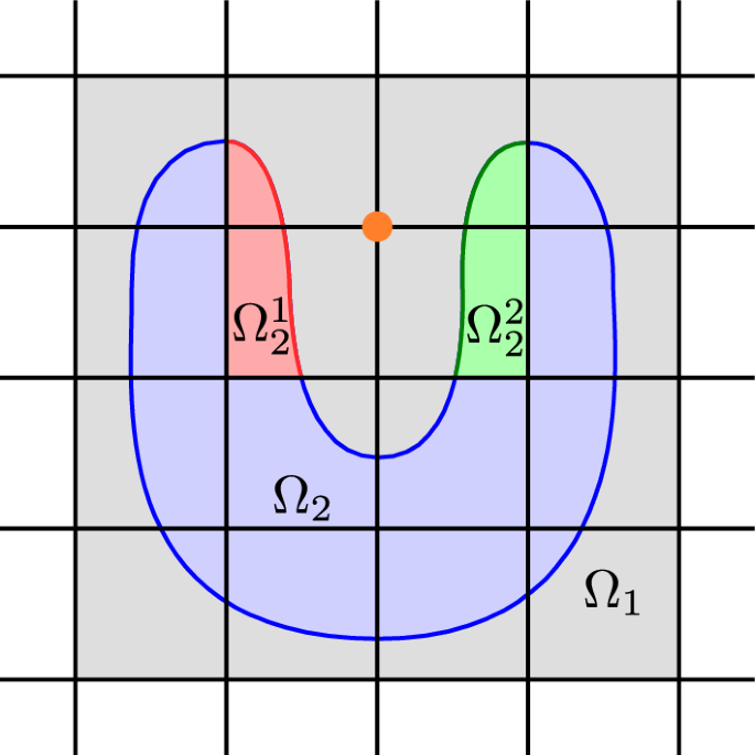
Visualization of a background mesh with a solid and fluid phase, and , respectively. Inside the fluid subdomain, , the linear basis function at the node marked in red is enriched such that each of the two domains and are interpolated by independent coefficients
For intersected elements, a geometry-aligned integration mesh is created to integrate one material phase at a time. Note that the quality of the integration mesh may be poor as it is only used for integration but not for interpolation purposes. The loose requirement on the mesh configuration allows for fast and robust mesh generation. The mesh generation used in this study is based on the background mesh splitting algorithm described in Villanueva and Maute (2014) and Noël et al. (2022).
3.2 Nitsche penalization
The Dirichlet boundary conditions on the fluid are enforced in weak form through Nitsche’s penalization method, introduced by Nitsche (1971) and adapted to fluid mechanics by Bazilevs and Hughes (2007).
In this study, the velocity vector is prescribed to along the boundary , which includes a subset of the outer boundary, , and the fluid–solid interface, . The contributions of the Nitsche penalization to the velocity and pressure residuals are as follows:
where is the outward pointing normal of the surface . The parameters and denote if the Nitsche formulation should be symmetric (in which case ) or skew-symmetric (). In this study, the symmetric Nitsche formulation is used. The additional term in the contribution to the velocity residual is weighted by the factor which is needed for stability purposes and provides explicit control over the strength with which the boundary conditions are enforced. The penalty factor, , is computed from the user-defined penalty parameter, , as well as the length of the interface within an element, h, the fluid viscosity and mass density, and , respectively, the velocity, u, as well as the Brinkman penalization term :
This formulation is inspired by the one used by Schott et al. (2015); the inverse permeability term is added to account for the body forces due to the Brinkman term, analogously to the term used to account for inertia forces in transient flow problems, see Schott et al. (2015). In this work, the user-defined penalty parameter is set to .
Imposing inlet boundary conditions might cause additional instabilities. This is alleviated by adding an upwinding term, , to the residual:
where the upwinding parameter is set to , as suggested by Schott and Wall (2014).
3.3 Stabilization of the weak form
Instabilities arise in the weak form of the Navier–Stokes equation (4) if the same interpolation is used for velocity and pressure and due to the convective term in the velocity residuals. In this study, the weak form is stabilized by the Pressure Stabilizing Petrov Galerkin (PSPG) and Streamline Upwind Petrov Galerkin (SUPG) stabilization schemes from Tezduyar et al. (1992), resulting in the following and contributions to the velocity and pressure residuals, respectively:
where and are the strong form residuals for the momentum and continuity equations, respectively (3). The stabilization parameters and are evaluated as suggested by Taylor et al. (1998) and Whiting and Jansen (2001). The inverse permeability, , is included in the stabilization parameters, as suggested by Alexandersen et al. (2014):
The parameter, , is set to 36, as suggested by Whiting (1999). The contravariant metric tensor, G, depends on the parametric coordinates of the background element, , and is summed over the number of considered dimensions, :
3.4 Ghost stabilization
The face-oriented ghost stabilization scheme is employed to alleviate issues due to background elements, which are cut such that the support of some basis functions along the fluid–solid element is small relative to basis functions with full support. The stabilization penalizes jumps in the gradients of the state field across the facets connecting cut elements with the interior of the fluid domain, as suggested by Burman (2010) and Burman and Hansbo (2014).
The set of ghost-stabilized facets contains the facets of cut elements that separate the two adjacent fluid domains, and . The normal of the facet is defined as the outward normal on the element , from which it follows that . The contribution is computed for each face being a member of , the total number of facets being . For details, see Noël et al. (2022).
The ghost stabilization formulation proposed by Schott and Wall (2014) is revisited to consider the inverse permeability contributions. As for the Nitsche penalization, the inverse permeability, , is included analogously to the inertia term for transient problems. The ghost stabilization leads to the following contributions to the velocity and pressure residuals:
where the superscript o is the interpolation order, which in the present work is , as linear B-splines are used. The ghost penalty factors are set to , as suggested by Burman and Hansbo (2014). The jump operator describes the jump of a quantity across a facet, from the element to , .
3.5 Demonstration of XFEM stabilization with Brinkman penalization
A simple verification problem is studied to test the formulation implementation of the Navier–Stokes equation with the Brinkman penalization using XFEM. For this purpose, a two-dimensional channel inspired by results from pipe-bend optimization problems is considered. The computational domain and dimensions are shown in Fig. 3, where the XFEM approach cuts out the inlet and outlet channels and the square area connecting them. The area around the bend connecting the inlet and outlet channels is defined as solid represented by the Brinkman model.
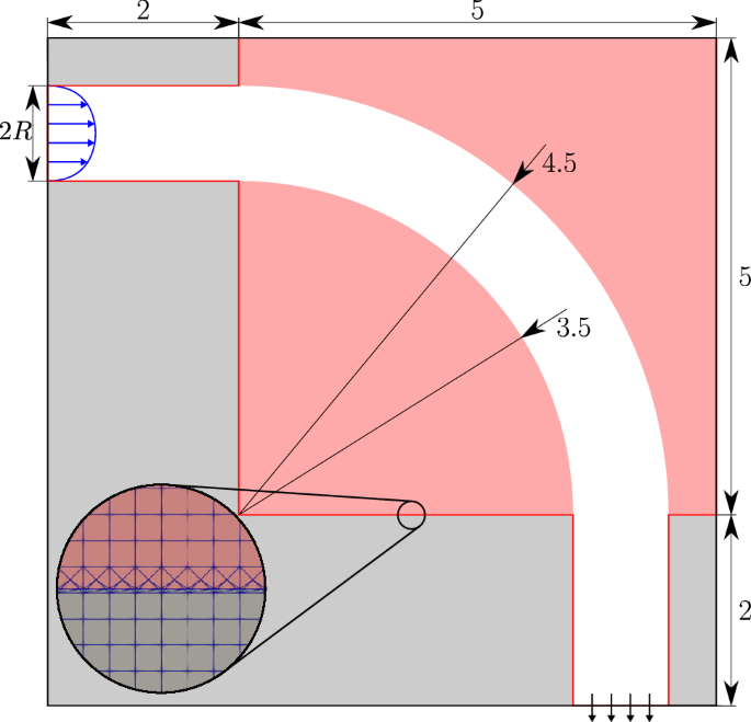
Setup of the pipe-bend-inspired channel, used to verify the implementation of XFEM with the Brinkman approach. The red areas are represented as solids using the fictitious solid approach by setting a high inverse permeability; the white area is pure fluid (i.e., ), and the gray areas represent the solid phase omitted in the XFEM analysis. The interface with cut interfaces is shown in red. The inset shows the integration mesh on a part of the cut interface
The computational domain is discretized using square elements of side length 0.07. The elements are not aligned with the fluid-void and solid-void interfaces; thus, background elements are cut along these interfaces.
The Reynolds number is set to and defined as
where the reference length is set to the radius of the inlet, , the density to , and the dynamic viscosity to (note that all quantities are given in self-consistent units). The inlet boundary condition is a parabolic velocity profile, scaled such that the average inlet velocity (the reference velocity) is . No-slip boundary conditions are prescribed on all boundaries except for the inlet and outlet.
In the following, the need for the inverse permeability terms in Nitsche’s method (8) and in the ghost stabilization (13) is demonstrated by considering four cases. The Nitsche method is chosen to be of the symmetric type in both cases by setting in (7). In all cases, the solid area outside the quarter circle channel is modeled by setting the inverse permeability to ; within the channel it is set to .
The velocity and pressure fields for the computations with and without the inverse permeability terms in the Nitsche and ghost stabilization formulations (all four cross combinations) are shown in Fig. 4. It is noted that stability issues prevent the solver from converging for the case, where the inverse permeability terms are omitted from the ghost stabilization and Nitsche formulation, shown in Fig. 4a and e, and the relative discrete residual stagnates around after 75 iterations. In the other three cases, where either one of the contributions or both are included, the Newton solver converges, and the corresponding final relative discrete residual norms and mass balances are shown in Table 1. The velocity and pressure fields obtained when only including the inverse permeability in the ghost stabilization are shown in Fig. 4b and f, respectively, and in Fig. 4c and g when the contributions are only included in the Nitsche penalization. The velocity and pressure fields obtained when the inverse permeability is included in the ghost stabilization and the Nitsche formulation are shown in Fig. 4d and h, respectively.
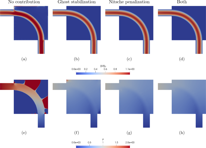
Verification test case of a pipe bend with cross combinations of the inverse permeability contributions in the Nitsche penalization and ghost stabilization. The velocity and pressure fields are shown in a–d and e–h, respectively. a and e show the fields when neither contribution is included, b and f show the fields when including the inverse permeability contribution in the ghost stabilization, c and g show the fields with the inverse permeability contribution included in the Nitsche penalization, and finally d and h show the fields with the inverse permeability included in both the Nitsche and ghost formulations
The test case highlights the importance of including the inverse permeability terms in the Nitsche penalization (7) and ghost stabilization (13). In Fig. 4a and e, where none of the inverse permeability contributions are included, fluctuations, spillage, and leakage appear in the velocity field near the wall, indicating an unstable numerical scheme. Note that these are the regions, where Nitsche’s method and the ghost stabilization are applied. Unphysical pressure fluctuations are also observed in this case. In Figs. 4b and 4f, where the inverse permeability contribution is included in the ghost stabilization but omitted from the Nitsche penalization, the velocity field does not appear to have any spurious modes. This is, however, not the case for the corresponding pressure field, where unphysical checkerboard-like patterns are observed along the boundaries (especially along the upper and right walls), indicating an unstable numerical scheme. In Fig. 4c and g, the inverse permeability contribution is included in the Nitsche penalization term but omitted from the ghost stabilization; in this case, no unphysical modes are observed in the solution. Finally, in Fig. 4d and h, both inverse permeability contributions are included, leading to a solution with no artificial modes. The comparison of the mass balances listed in Table 1 shows that including both contributions also leads to the most accurate mass balance among all configurations studied. Note that the mass balance could be further improved by increasing the Nitsche penalty and mesh refinement. Having both contributions included in the formulation improves the conditioning of the problem.
4 Optimization
The PDE-constrained optimization problem considered in this paper can be written in general form as follows:
The design vector, , collecting the design variables , is optimized, such that the variables are within the lower and upper bounds, and , respectively. For a given design , the corresponding state variables are computed such that the discrete residual is . The nested formulation implicitly satisfies this equality constraint (to the non-linear solver tolerance). The objective function is minimized, while m constraints, , have to be satisfied.
The Globally Convergent Method of Moving Asymptotes (GCMMA) by Svanberg (2002) is used to find a feasible minimum. The optimization method is applied with no inner iterations. The design sensitivities are computed by the adjoint method.
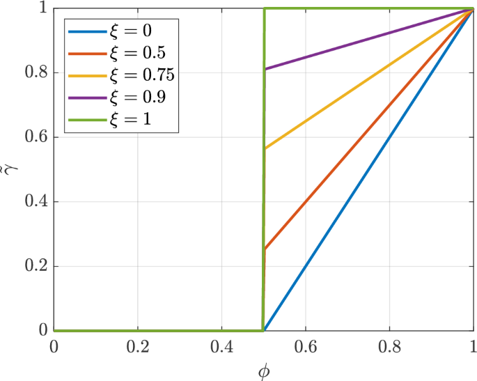
Relation between the design variable value, , and the shifted density variable for different shifting values, , for the case where , , and
4.1 Density shifting strategy
As the density field is used only for hole nucleation, its influence on the fluid model is sought to be eliminated once the topology of the design has been obtained (Barrera et al. (2020)). Therefore, after initial design iterations, the density field is shifted over iterations, such that after the shifting is completed, the shifted density field yields . This is achieved by ramping the parameter from after design iterations to after iterations. The resulting shifted density field at the current design iteration, N, is given by
Hence, as initially , the optimization starts with and when , , signifying that the density method has been eliminated. The parameter enables the transition from a hybrid density level-set method to a pure level-set approach. In Fig. 5, the shifted density variable is shown as a function of the design variable, , for a set of ramping parameters . Defining the interpolation of the ramping parameter by a quadratic polynomial (16) allows for fine-tuning the effect of the density shift such that the shift is initially small, while the main part of the shifting occurs in the later stages of the continuation. Note that the discontinuity in the function, as it is shown in Fig. 5, can be disregarded, as the density function is defined only in the fluid phase, , where .
4.2 Volume and permeability interpolation
The volume fraction, v, used to compute the current design’s fluid volume, is interpolated linearly from the shifted density variable, .
The inverse permeability is computed from the shifted density variable using the RAMP interpolation scheme (Stolpe and Svanberg (2001)):
where the penalization parameter q describes the non-linearity of the interpolation. If , the interpolation is linear.
4.3 Problem setup
The objective function is composed of a quantity that is sought minimized, , and two regularization functions: one for the level-set field, , and the other for the perimeter, , with their respective weights and :
In the optimization problems considered in this work, the minimized quantity, , is the fluid power dissipation, normalized with the initial power dissipation :
The regularization functions are discussed in Sect. 4.4.
For configurations with multiple outlets, constraints are imposed to control the fluid flow through these outlets. A target outflow is defined for each outlet, denoted by the index i. The actual outflow through the corresponding outlet is computed by
where is the outward pointing normal. Two constraints are enforced for each outlet, ensuring that the outflow through the outlet is within an allowable relative deviation, :
Setting relaxes the constraint. An alternative formulation of the constraints can also be formulated with one constraint per outlet by squaring the outflow deviation. However, the formulation with two constraints was found to be more stable in the context of the present work. Note that the sum of the target outflows should match the inflow.
This study also considers a problem where the velocity distribution at the outflow port is required to match a given spatial profile. In this case, the following flow distribution constraint is enforced, penalizing the deviation of the outlet velocity from the target, , with an allowable deviation, :
A volume constraint on the fluid phase is enforced on all optimization problems, requiring the fluid volume to be less than the maximum admissible volume, . The fluid volume is computed by integrating the volume fraction, , over the fluid phase, . The constraint is formulated as follows:
4.4 Regularization
The iso-contour of the level-set field defines the shape of the solid–fluid interface. The values of the level-set field away from the interface and the spatial gradients of the level-set field along the interface have no physical relevance. These values and gradients may suffer from spurious oscillations, which can hamper the convergence of the optimization process. To avoid this issue, the level-set field needs to be regularized.
While the design variable is coupled to the relative density (and hence the inverse permeability) which provides regularization within the fluid, the design variable in the solid domain still calls for some regularization. This also becomes the case for the fluid domain once the shifting strategy is terminated and the density field’s regularization is eliminated.
The level-set field regularization scheme proposed by Geiss et al. (2019) is used to alleviate spurious oscillations. The method builds on creating an ideal representation of the level-set field, , which conserves the same interfaces as the actual level-set field, . The target field, , is constructed from a signed distance field which is truncated and scaled. The target field has a uniform gradient close to the interface and the value of either an upper or lower bound away from the interface. The signed distance field is computed by the heat method of Crane et al. (2017), which relies on solving one backward-Euler heat diffusion time step and a Poisson problem both of which are solved using XFEM. The level-set field is regularized through a penalty term that measures the difference between the actual and the target field and the difference between their spatial gradients. The penalty term is constructed as
The normalization factor is found as the regularization value at the first iteration, where the density shift is initiated.
The weights for the penalty term, and , for the LSF value and gradient, respectively, are defined such that the gradient penalty dominates close to the interface and the value far away from it. The reader is referred to Noël et al. (2020) for a detailed discussion of the penalty weights.
A perimeter penalty is also augmented to the objective function, as suggested by Haber et al. (1996). This penalization aims to prevent irregular geometric features from appearing due to numerical artifacts in the finite element formulation. The penalization reads
where is the perimeter in the first design iteration by which the regularization is normalized.
4.5 Sensitivity analysis
The sensitivity of a generic function with respect to the design description is obtained by solving the adjoint problem for the Lagrange multiplier :
The sensitivities of the function are then retrieved by
The semi-analytical method introduced by Sharma et al. (2017) is used to compute the chain rule terms with respect to the design variables.
In pure level-set methods, non-zero sensitivities for the power dissipation and constraints presented in Sect. 4.3 are only found along the interface between the fluid and solid. In density methods, however, non-zero sensitivities are found throughout the design domain. In the presented method, the density method is only applied in the fluid phase of the optimization. Hence, non-zero sensitivities are only found inside the fluid domain (while ) and at the interface between fluid and solid.
5 Optimization studies
In the following, the density-based hole-seeding approach for level-set flow topology optimization is studied with four examples. First, the well-known pipe-bend example is considered in two dimensions to visualize and validate the methodology. Then, flow diffusers are considered in two dimensions; the design goal is to generate an outlet flow with a uniform velocity profile. Flow manifolds are optimized in both two and three dimensions. These devices aim to distribute the inlet flow evenly across multiple outlets.
Table 2 lists the optimization parameter settings for the examples. In all cases, the level-set regularization weight, , is ramped up linearly along with the shifting parameter . The corresponding normalization for the level-set normalization, , is set to the regularization penalty value when the density shift continuation starts. All other normalizations are set in the first design iteration.
5.1 2D Pipe bend
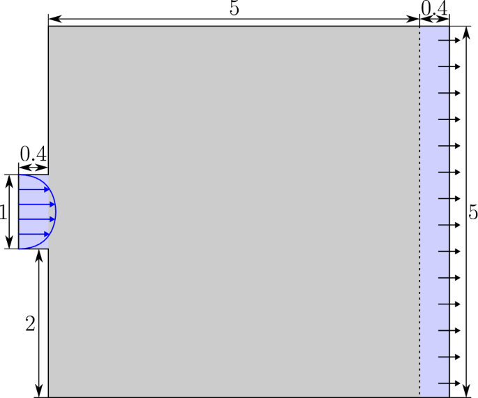
The presented hole-seeding method is first tested on a two-dimensional pipe-bend problem. The layout of the optimization problem is seen in Fig. 6. The design domain is of dimensions . Additionally, channels of length 2 with prescribed fluid phase and are placed at the inlet and outlet. These channels are not subject to optimization. A parabolic velocity profile is imposed at the inlet of the upper left channel. The background mesh discretizes the domain into square elements with side length 0.1.
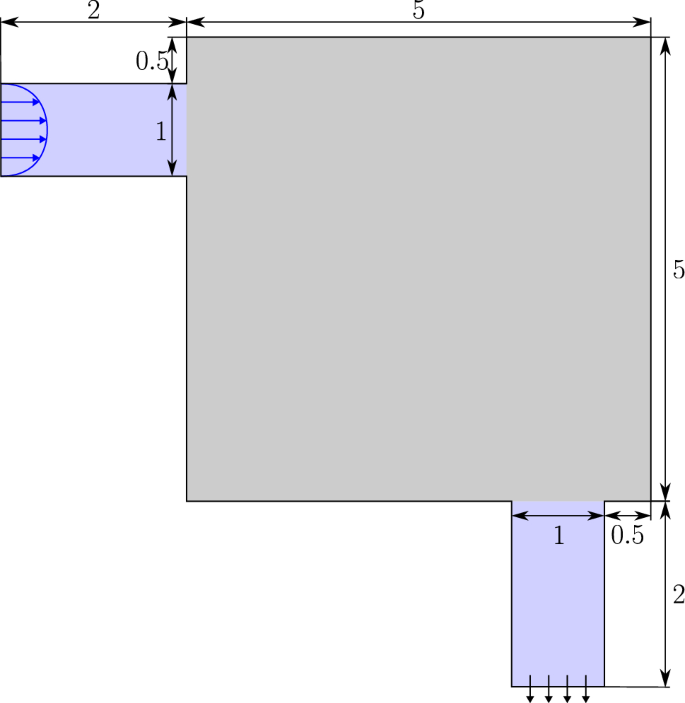
Layout of the pipe-bend optimization example. The gray area is the optimization domain, while the blue channels are prescribed to fluid
In this example, only the volume constraint (23) is considered, in addition to the box constraints on the design variable. The maximum volume is of the design domain; the fluid volume of the inlet and outlet channels is not considered in the formulation of this constraint.
The problem is run for two Reynolds numbers, and , by setting the average inlet velocity to and , respectively. The dynamic viscosity is set to and the fluid density to in both cases. Note that throughout this work, all fluid properties, lengths, and velocities are given in self-consistent units. The reference length is the inlet radius, .
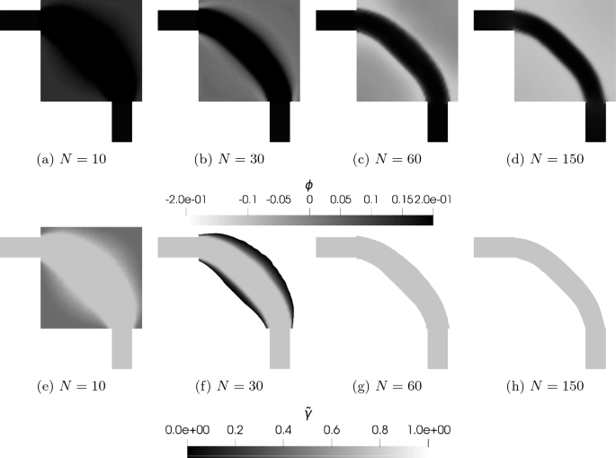
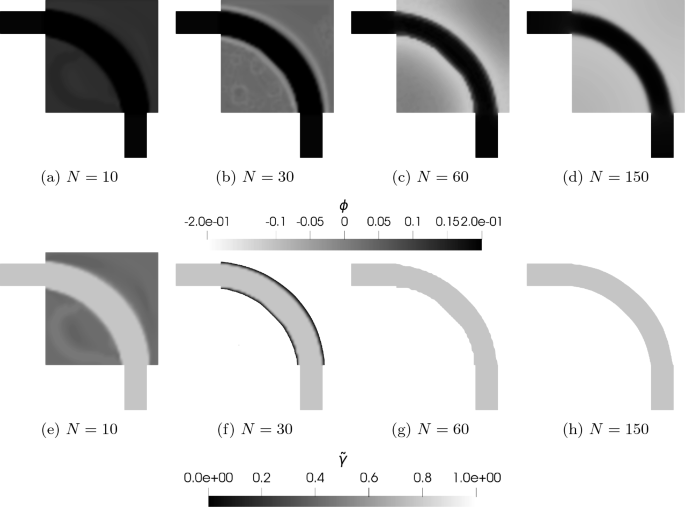
Design evolution of the design variable, , (a–d) and evolution of the corresponding shifted density fields, , (e–h) for the pipe bend optimized with a Reynolds number . Final objective
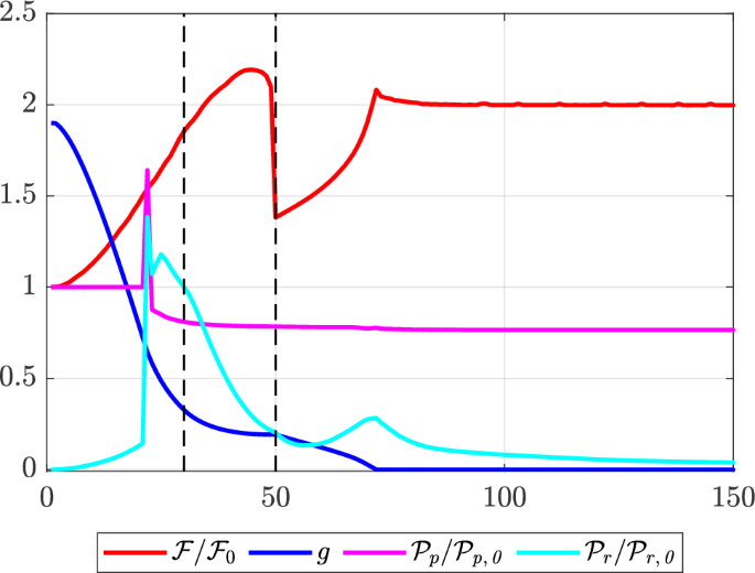
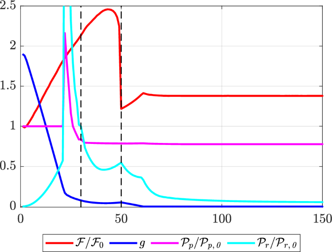
Optimization evolution of the pipe bend with . The fluid power dissipation and two regularization penalties are normalized. Dashed vertical lines show the interval of the density shift continuation
Figure 7 provides snapshots of the design variable , as well as the shifted density field, , for the case where , at different design iteration steps and in the final design. The snapshots show that the design variable behaves as expected for a density-based optimization process in the initial design stages. This is also observed in the shifted density field, which is still an offset and rescaled version of the design variable at this stage of the optimization process. In the following snapshot of the design iteration, the design variable has moved below the threshold value in parts of the design domain. The channel is padded with some material with intermediate density values, highlighting that the method still is hybrid at this state. After 60 design iterations, the shifting parameter has reached its final value, . This is highlighted by the pure fluid density field observed at this stage. The optimization process was terminated after 150 design iterations, where the design was visually converged. The final design consists of an almost straight channel connecting the inlet and outlet channels. The slight curve in the channel, opposite the completely straight channels obtained for Stokes flow by Borrvall and Petersson (2003), is attributed to the use of the Navier–Stokes model which accounts for inertial effects. The corresponding design field goes from the lower bound in the far-field solid domain to the upper bound in the far-field fluid domain. The transition from the lower to the upper bound is smooth near the interface. This desired feature is attributed to the regularization scheme discussed in Sect. 4.4.
Design evolution of the design variable, , (a–d) and evolution of the corresponding shifted density fields, , (e–h) for the pipe bend optimized with a Reynolds number . Final objective
Optimization evolution of the pipe bend with . The fluid power dissipation and two regularization penalties are normalized. Dashed vertical lines show the interval of the density shift continuation
The evolution of the fluid power dissipation, the volume constraint, and the level-set and perimeter regularization penalties in the optimization process are depicted in Fig. 8. The evolution of objective and constraint values shows that reducing the fluid volume to meet the constraint directly counteracts the objective of minimizing the fluid power dissipation. The two regularization penalties for the perimeter and level-set field, and , respectively, spike when the design field first drops below its threshold value, , creating a solid phase in parts of the design domain. During the continuation of the density shift parameter, , the volume constraint does not drop significantly; however, the fluid power dissipation increases during the corresponding optimization steps. This might be linked to the density shifting increasing the density values of points with intermediate density values, requiring the volume of the fluid phase, , to drop. Once the density shift continuation is finished, a significant drop in the fluid power dissipation is observed. This is linked to the elimination of intermediate densities along the channel’s boundaries. As the volume constraint is pulled toward feasibility, the dissipation increases and slightly drops after a feasible design is obtained.
As for the case with , Fig. 9 shows the design representations at multiple optimization steps for the case with .
The snapshots of the design iteration show that a curved bend is already outlined from the early stages of the design history. After 30 iterations, just before the start of the ramping of the shifting parameter , the design variable has dropped below the threshold in the area outside the curved bend, such that the fluid domain now consists of the bend, padded by a very thin layer of intermediate relative density values. After the density shift continuation has finished, the bend is more clearly defined, and the design field decreases to the lower bound in the solid phase, away from the interface. The wall also seems more regularized than is the case for at this point in the optimization evolution. This might be due to the flow with a higher Reynolds number being more sensitive to the boundary of the channel due to the convective effects. The final design, obtained after 150 iterations, consists of a pure fluid curved channel connecting the inlet and outlet with smooth boundaries.
The design evolution for the case with is shown in Fig. 10. The fluid power dissipation and perimeter regularization are normalized with their values in the first design iterations. The level-set field regularization, , is regularized with its value in the design iteration, where it starts to be incorporated into the objective function. A spike in the two regularization functions is observed after design iterations, corresponding to where the design variable drops below its threshold value, , creating the solid phase. During the continuation of the parameter, advancing the density shift between the and design iteration, a slight increase in the volume constraint is observed. This can be linked to the shifting strategy, which increases the volume taken into account for the constraint by shifting the density field.
This also explains the slightly increasing value of the fluid power dissipation. After the density shift continuation is finalized, such that no non-zero inverse permeabilities are left in the fluid domain, the fluid power dissipation drops significantly. This is because the channel formed by the optimization is no longer padded with intermediate densities. Just after the significant drop, the fluid power dissipation increases again. This is attributed to the volume constraint being slightly violated due to the density shift continuation.
Generally, the pipe bend yields an almost straight connection from the inlet to the outlet channel when and a clear curved bend when . These results coincide well with the results found in the literature, notably, Gersborg-Hansen et al. (2005).
This example demonstrates the basic functionality of the proposed hole-seeding method. However, the optimization problem, i.e., minimizing power dissipation subject to a constraint on the fluid volume, exhibits good convergence. The topology of the flow channel forms early in the design process and only the shape of the channel walls is fine-tuned after that. This evolution of topology and shape aligns well with the proposed hole-seeding method, transitioning from density-based to level-set optimization. The following examples consider problems that lead to less benign design evolutions and pose larger challenges to the proposed method.
5.2 Diffuser for uniform outflow distribution
A diffuser device is optimized such that the spatial distribution at the outflow port matches a described uniform profile. Such devices can be crucial for heat exchangers, where the inlet flow profile, created by an upstream diffuser, can significantly affect the performance. The setup of the optimization problem is shown in Fig. 11. The computational domain consists of a small inlet channel, which connects the inlet port on the left with a wide design domain. A thin layer of fluid is placed between the design domain and the outlet port on the right to avoid any solid being connected to the outlet. The computational domain is discretized by a background mesh consisting of square elements with side length 0.07.
Domain configuration for the diffuser optimization example. The gray area is the optimization domain, while the white areas are fixed to fluid
The objective of the optimization is to minimize the fluid power dissipation while enforcing a constraint on the fluid volume and on the spatial distribution of the horizontal flow velocity across the outlet (22). The target flow profile is constant, evenly distributing the inlet flow across the outlet. The maximum admissible deviation from the target metric is set to . This relatively large number is chosen as a boundary layer will be present near the outlet edges, meaning there will be unavoidable deviations from the target velocity. The outflow distribution problem is notoriously difficult to solve with the density method, as it tends to take advantage of the porous nature of the flow in the solid, which distributes the flow but does not act like a solid in these cases.

Design evolution of the design variable, , (a–d) and evolution of the corresponding shifted density fields, , (e–h) for the diffuser optimized with a Reynolds number . Final objective
A parabolic velocity profile with the center velocity is enforced at the inlet, leading to a Reynolds number of , as the fluid density and viscosity are set to and , respectively. The target velocity at the outlet is set to . The maximal admissible fluid volume is set to of the design domain, which does not include the fluid volume in the inlet channel and outlet region.
The distribution constraint is computed as the deviation of the velocity; however, the fluid volume is a conserved quantity, rendering the constraint highly non-linear. Due to this behavior, the design variable’s move limits for GCMMA are set to per design iteration. The topology optimization is run for 450 design iterations, after which it is visually converged.
Snapshots of the design, , and shifted density field, , respectively, are shown at different design iterations in Fig. 12. The material distribution at design iteration 10 suggests that intermediate densities near the outlet benefit the constraint on the even outflow profile. The porous region equalizes the flow profile.
Density distributions representing pure fluid are observed in later design stages, as these are beneficial for the objective. However, in the center of the diffuser, intermediate density values are still present for the reason stated above. At two solid islands have formed within the inverted nozzle shape. These two features redirect the flow toward the upper and lower edge of the design domain.
As the density shift continuation is finished, more islands have appeared. Two center islands form a center channel with enough flow resistance to prevent the main part of the fluid from flowing through it. On the lower and upper sides, additional islands have also formed.
The pure level-set topology optimization process has a large influence on the final design, as there are four islands left in the final design, as seen in snapshots for . The center islands are now small, and the ones on the sides of the domain have grown significantly.
The design history is shown in Fig. 13. The design history highlights the sensitivity of the uniform flow distribution constraint to even small design changes. This is likely linked to the complex interplay between the requirement to create a desired flow profile and the conservation of mass. Design changes taken to meet the target velocity in one location will likely counteract the velocities being close to the target in another location.
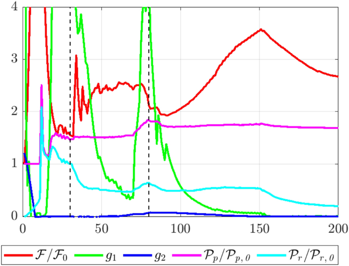
Optimization history of the diffuser with . The first constraint, , is the distribution constraint, and is the volume constraint. The fluid power dissipation and two regularization penalties are normalized. Dashed vertical lines show the interval of the density shift continuation
The velocity field of the optimized diffuser is shown in Fig. 14, where it is seen how the widening shape of the fluid domain and the four islands let the flow move to the sides of the fluid domain. Downstream of the islands, the velocity field diffuses to a more even state, satisfying the distribution constraint.
In Fig. 14, it is also observed that the design is slightly asymmetric. This is attributed to the imperfect convergence of the Newton solver, creating a slightly unsymmetric state field, which, in turn, leads to unsymmetric sensitivities.
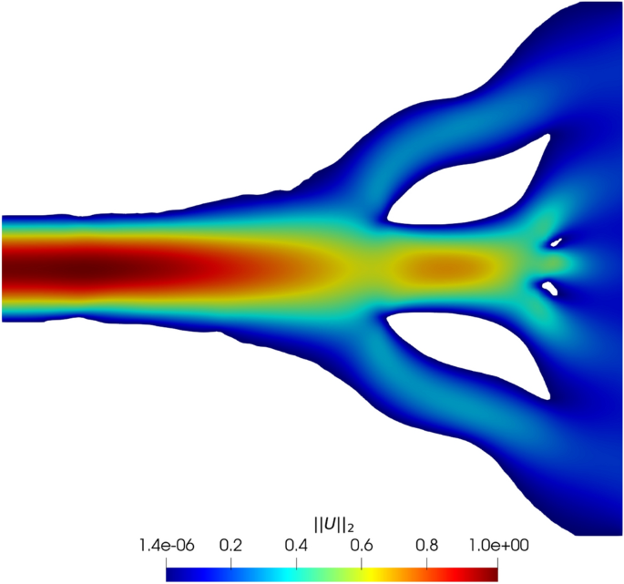
Velocity magnitude in the optimized diffuser with . The inverted nozzle shape and two obstacles inside the diffuser distribute the flow evenly across the outlet
The outlet flow profile in the optimized fluid manifold is shown in Fig. 15. From the profile, it is observed that the flow rate near the lower and upper boundaries undershoots and that it overshoots in the middle of the domain. Furthermore, the influence of the fluid islands in the optimized design is seen through the velocity magnitude peaks over the design cross-section.
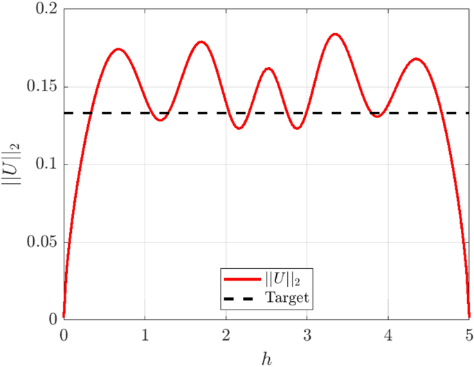
Outlet flow profile in the optimized flow diffuser manifold. The obtained outflow is shown by red and the target by the black dashed line
This example demonstrates that the proposed hole-seeding method is also successful for problems where using intermediate densities in some regions of the design would provide an advantage. The density shift eliminates all intermediate densities, and the level-set field shapes the fluid domain in response to removing intermediate densities. This example also shows that the pure level-set part of the optimization can have a larger role than only smoothing out the boundaries, as the design is changed considerably in the final design stages.
As the previous example, also this problem has one inlet and one outlet port. This provides a strong bias for a simple overall flow path. Thus, one could consider this problem also to be a benign case for the proposed method. The following example will address this issue.
5.3 2D Flow distribution manifold
The density-based hole seeding is now applied to a two-dimensional flow distribution problem considering the manifold shown in Fig. 16. The problem consists of evenly distributing the flow from the inlet throughout five different outlets. In addition to the volume constraint (23), ten constraints, two for each outlet, are enforced on the outlet flow rates (21). The target flow rate, , is set to of the inlet flow rate for each outlet, and the admissible deviation is . The volume constraint states that no more than of the design domain can belong to the fluid subdomain, which helps to regularize the optimization problem. In the present work, the geometry parameter is set to ; see Fig. 16. The background mesh consists of square elements with a side length of 0.1. The optimization problem is studied for two different inflow velocities.
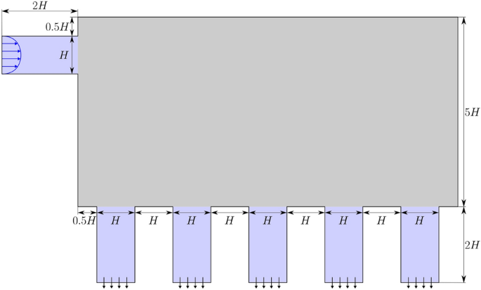
Domain configuration for the 2D flow distribution manifold optimization example. The gray area is the optimization domain, while the blue channels are fixed to fluid
The optimization is first carried out at a low Reynolds number, , which is achieved by setting the fluid density and dynamic viscosity to and , respectively. The reference length is set to the inlet channel radius, , and hence the average velocity of the inlet, which is used as the reference velocity, is set to .
The optimization is run for a total of 150 design iterations, after which the optimization is visually converged. Snapshots of different stages of the optimization process are shown in Fig. 17. These snapshots show again that the optimization in its early stages behaves like a pure density-based approach, as only material with intermediate densities is placed in the design domain. At the start of the continuation of the density shift, after design iterations, the level-set field has dropped below the threshold in some parts of the design domain. However, spatial oscillations of the density field around the threshold lead to many small islands and holes. Furthermore, some greyscale is observed in the density field near the branching of the channels. This greyscale material creates flow resistance, which facilitates even distribution of the flow. After the continuation of the density shift is complete, the irregularities near the boundary of the primary fluid structure disappear, and the level-set field is regularized. The regularization schemes on the perimeter and level-set field ensure that the islands are eliminated.
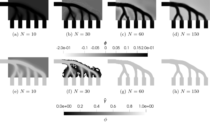
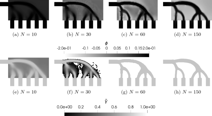
Design evolution of the design variable, , (a–d) and evolution of the corresponding shifted density fields, , (e–h) for the fluid manifold optimized with a Reynolds number . Final objective
A second flow manifold optimization is run with a Reynolds number of , where the average inlet velocity is set to and all other parameters are kept at the same level as in the previous case. Snapshots from this case are shown in Fig. 18. The snapshots show a similar behavior to the case with . In the snapshot from the design iteration, the same behavior as previously observed can be seen, where small islands form around the structure, due to oscillations in the design field. These areas have a lot of intermediate relative densities throughout, in contrast to the previous examples where the main flow path emerged very early in the optimization process. Here, the flow path is less clear which causes the continuation strategy to have a stronger influence.
Design evolution of the design variable, , a–d and evolution of the corresponding shifted density fields, , e–h for the fluid manifold optimized with a Reynolds number . Final objective
A noticeable difference is observed in the optimized designs of the two flow manifolds, optimized for Reynolds numbers of and , respectively. The velocity distribution in the two designs is shown in Fig. 19. The channels in the manifold optimized for are more curved than in the design optimized with a Reynolds number of . These curved features are beneficial at higher Reynolds numbers, as observed for the pipe bend. Hence, a flow manifold for a higher Reynolds number also possesses more curved features. Both designs branch the channel for the two outlets closest to the inlet similarly. For the three outlets furthest away from the inlet, the two designs differ, however. In the design optimized for the low Reynolds number, , the channels going to the outlets branch off an almost straight channel going from the first branch for the first two outlets to the outlets furthest away from the inlet. In the design optimized for the higher Reynolds number, however, an apparent bend is formed from the location of the branch to the first two inlets to a location above the outlet, the second furthest away from the inlet. At this location, the channel branches into three, each going to its respective outlet.
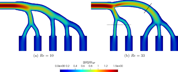
Distribution of velocities normalized by the reference velocity in the flow manifolds optimized with Reynolds numbers of a and b . The solid and dashed lines in b indicate the curves along which the plots in Fig. 20 are done
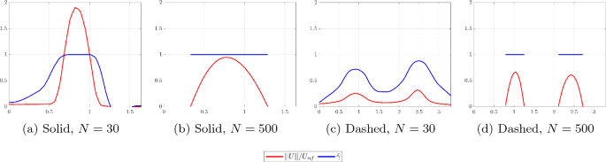
Velocity and density profiles in the manifold design with , along the lines displayed in Fig. 19b. a and c shows the profiles after 30 design iterations, and b and d in the final designs
Comparing the results presented above suggests that as the momentum in the flow gets higher, it becomes more beneficial to have a manifold consisting of a single channel which splits close to the different outlets, as it is observed for in Fig. 19b. For the case with lower momentum in the flow, channels going to the different outlet ports branch off earlier.
For , the density and normalized velocity profiles along the lines shown in Fig. 19b are shown for the design after 30 iterations and the final design in Fig. 20. From the cuts in the design obtained after 30 design iterations, it is seen that there is some flow through the areas with intermediate relative density values. Furthermore, at this design stage, it can be difficult to extract where the boundary between fluid and solid is. In the final design, the relative density is in the entire fluid domain. Hence, the velocity profile here goes to zero at the interface between the fluid and solid, , and has a parabolic shape.
5.4 3D Flow distribution manifold
To illustrate the applicability of the proposed method to three dimensions, a three-dimensional fluid manifold is now optimized. The optimization formulation is similar to the one used in Sect. 5.3, where the objective is to minimize the fluid power dissipation (19), while constraints on the outflow across the five outlets, , are imposed with the formulation from (21). The target outflow for each outlet is set such that even distribution among the outlets is sought, i.e., .
The design domain consists of a cube of dimensions , with passive fluid cylindrical channels of diameter 1 and length 2 attached to the center of each face of the design domain. For simplicity, only a quarter of the design domain is modeled and optimized, as shown in Fig. 21, where the two planes delimiting the considered quarter are shown on the total domain. Symmetry boundary conditions are considered along these planes. The target outflow rates are adjusted to account for only analyzing a quarter of the domain. The quarter domain is discretized by a background mesh consisting of cubes with a side length of 0.058.
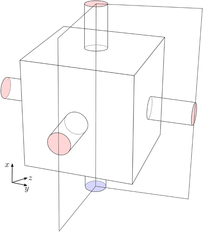
Geometry of the three-dimensional flow distributor optimization. The blue surface indicates the inlet and the red surfaces are the outlets, among which the flow will be evenly distributed. The design domain is the cube, while the in- and outlet channels are fixed to fluid throughout the optimization. Note that there also is one outlet on the back side of the design domain
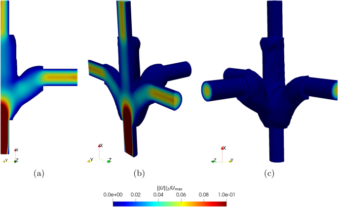
Optimized 3D flow manifold for a Reynolds number of colored by the normalized velocity magnitude. Note that the velocity overshoots the applied colormap. The domain is mirrored in b and c
The optimization is run at a Reynolds number of , which is obtained by setting the viscosity and density to and , respectively, and the average inlet velocity to , over a parabolic profile. The other optimization parameters are shown in Table 2.
The obtained design is shown in Fig. 22, where a branching toward all the outlet channels is observed as expected. A necking is observed in the channel connecting the outlet channel located on the opposite side of the inlet. This feature limits the flow into the outlet opposite the inlet, ensuring an even distribution as it forces flow to go through the outlets at the sides. Furthermore, the channels connecting to the outlets orthogonal to the inlet are swept with the flow direction. This feature is both good for the power dissipation objective as well as for the distribution constraint.
6 Conclusion
This paper presents an optimization strategy that uses the density method in XFEM-driven level-set topology optimization to seed solid inclusions. Flow through porous solid is described by the Brinkman model with a spatially varying impermeability. The impermeability is defined in terms of a density variable within the fluid phase. The density distribution and the level-set function are both defined in terms of a design variable field. This approach allows for pure fluid initial designs and mitigates the need for seeding inclusions into the optimization domain. To obtain smooth designs, the design variable field is parameterized by quadratic B-splines on a mesh that is coarser than the one used for the flow analysis. To eliminate intermediate densities from the final design, the densities are shifted toward one in the course of the optimization process. This continuation strategy is crucial to transition from a pure density to a pure level-set method.
The flow is described by the incompressible Navier–Stokes equation which is discretized by a Heaviside enriched XFEM approach, where the velocity and pressure fields are discretized by linear B-splines. Numerical studies showed that including the inverse permeability terms in Nitsche’s method and the ghost stabilization is critical for the stability of the state evaluation using XFEM formulation. The added terms are scaled similarly to the inertial terms when including the time domain in the analysis.
For the pipe-bend optimization, results like those seen in the literature are obtained, where a pure fluid start guess is usually needed. In the diffuser example, where a diffuser was optimized for an even outflow distribution, changes in the topology of the design were obtained after the hole nucleation process was completed. The two following examples consider the optimization of two- and three-dimensional flow manifolds, where the flow is distributed evenly among multiple outlet ports to obtain designs that do not exploit porous media to distribute the fluid. The optimization studies show that the presented method circumvents the need to seed holes. The density shift continuation needs to be done slowly to prevent convergence to infeasible designs or weak local minima.
Future work could use the presented methodology for problems involving, for example, conjugate heat transfer. Leakage of fluid into the solid domain may be observed in density methods and is problematic for the performance evaluation of conjugate heat transfer applications and problems with a large pressure drop. The penetration creates a combination of convection and conduction, which would otherwise not be physically possible. Therefore, applying the presented method could circumvent these issues after the initial design stages, where the topology of the design is seeded using the density method.