Article Content

Abstract

We develop a symmetry-based variational theory that shows the coarse-grained balance of work inflow to heat outflow in a driven, dissipative system relaxed to the golden ratio. Two order-2 Möbius transformations—a self-dual flip and a self-similar shift—generate a discrete non-abelian subgroup of PGL(2,(5−−√)). Requiring any smooth, strictly convex Lyapunov functional to be invariant under both maps enforces a single non-equilibrium fixed point: the golden mean. We confirm this result by (i) a gradient-flow partial-differential equation, (ii) a birth–death Markov chain whose continuum limit is Fokker–Planck, (iii) a Martin–Siggia–Rose field theory, and (iv) exact Ward identities that protect the fixed point against noise. Microscopic kinetics merely set the approach rate; three parameter-free invariants emerge: a 62%:38% split between entropy production and useful power, an RG-invariant diffusion coefficient linking relaxation time and correlation length 𝒟𝛼=𝜉𝑧/𝜏, and a 𝜗=45 eigen-angle that maps to the golden logarithmic spiral. The same dual symmetry underlies scaling laws in rotating turbulence, plant phyllotaxis, cortical avalanches, quantum critical metals, and even de-Sitter cosmology, providing a falsifiable, unifying principle for pattern formation far from equilibrium.
Keywords:

non-equilibrium thermodynamics; entropy; criticality; branching and phyllotaxis; neural avalanches; Fibonacci anyons; rotating turbulence; galactic spirals; golden ratio universality class


1. Introduction

The golden ratio, 𝜑1.618, has been documented in phyllotactic leaf arrangements; branching patterns of trees, blood vessels, lightning, and river deltas [1,2,3,4]; logarithmic spirals in hurricanes and galactic arms [5,6]; power law exponents in rotating turbulence [7,8,9,10]; quasicrystals [11,12,13]; mass gaps of critical Ising chains [14,15]; band structures of twisted bilayer graphene [16,17,18]; Fibonacci anyons dimensionality [19]; avalanche statistics in cortical activity [20,21,22]; and more. Classical equilibrium thermodynamics, tied to isolated systems and static-state variables, cannot explain the ubiquity of spirals, branching, fractals or, scale-invariant kinetics across scales [23,24,25], and a unifying, model-independent, non-equilibrium principle explaining the golden mean universality class is yet to emerge [26,27,28,29,30]. Empirically, these systems share two attributes: (i) they are maintained far from equilibrium by continuous energy or matter influx (e.g., solar radiation, gravitational shear, biochemical energy) [25], and (ii) they exhibit nonlinear, irreversible dissipation (e.g., thermal conduction, radiative cooling, viscous dissipation, chemical enthalpy release) while maintaining coherent large-scale organization and optimal functionality [31].
In this work, we show that a single symmetry-protected variational principle—Dynamic Balance (DB)—forces any driven–dissipative system to relax towards the golden ratio. We define a dimensionless ratio–entropy flux field 𝛼(𝑡)–comparing two irreducible forms of energy: useful power inflow 𝐸˙ (reversible) and entropic heat outflow 𝑇𝑆˙ (irreversible). A large 𝛼 implies low dissipation; a small 𝛼 means the system overheats, leaving little energy to build or maintain structure. Most real systems develop negative feedback loops (physiological, hydrodynamic, or electronic) to prevent collapse or runaway behavior, thereby stabilizing their internal state [32]. For instance, excessive anabolism or catabolism harms living organisms, so metabolic circuits self-regulate through hormones and growth-factor inhibition [33]. Consequently, a driven system in a sustained non-equilibrium steady state will adjust 𝛼(𝑡) toward a constant, 𝛼, that optimally balances useful work against dissipation. Across scales, systems at 𝛼 exhibit hierarchical organization—smaller subsystems nested within larger ones—and scale-invariant, fractal dynamics. Therefore, we posit that this optimum is the golden ratio, 𝛼=𝜑.
From a group-theoretical perspective, every physical process is the result of a selection rule dictated by an underlying symmetry [34,35]. We show that two discrete Möbius maps 𝑆𝜑 (a self-dual involution) and 𝑇𝜑 (a self-similar recursive shift) acting on 𝛼, and realized microscopically by antisymmetric Onsager couplings [36,37,38] and cross-correlated noise in active media [39], respectively, generate a non-Abelian subgroup of PGL(2,(5−−√)). Requiring any strictly convex Lyapunov cost 𝑅(𝛼) to remain invariant under both maps singles out the unique stable fixed point 𝛼=𝜑. Microscopic details affect only transients, and the system dynamically self-organizes around the golden mean. This modular symmetry and convex geometry guide the entropy flux field, giving rise to Legendre dual flows and emergent conjugate pairs observed in all physical laws.

𝐒𝐲𝐦𝐦𝐞𝐭𝐫𝐲ModularDuality𝐆𝐞𝐨𝐦𝐞𝐭𝐫𝐲Convexity𝐃𝐲𝐧𝐚𝐦𝐢𝐜𝐬LegendreDuality𝐎𝐛𝐬𝐞𝐫𝐯𝐚𝐛𝐥𝐞𝐬
The paper is organized as follows: Section 2 states and proves the core theorem. Section 3 builds the gradient-flow PDE and extracts three parameter-free invariants (entropy split, 𝜉2Γ, and 45 spiral pitch). Section 4 shows that a discrete birth–death Markov model recovers the same continuum PDE limit, while Section 5 embeds the theory in a Martin–Siggia–Rose field integral and derives exact Ward identities that protect 𝜑 against noise. We close with cross-domain applications—turbulence, neuroscience, quantum criticality, and cosmology.

2. Mathematical Framework

Theorem 1.

Let 𝑆𝜑:𝛼Λ2/𝛼 and 𝑇𝜑:𝛼1+1/𝛼 be two Möbius transformations generated microscopically by
  • 𝑆𝜑: antisymmetric Onsager exchange 𝐿𝐴𝐵=Λ2𝐿𝐵𝐴
  • 𝑇𝜑: cross–correlated noise source source 𝜉𝐴𝜉𝐵
These two maps generate a discrete, non-Abelian subgroup of 𝑆𝜑,𝑇𝜑PGL(2,(5−−√)). Define the minimum smooth and strictly convex Lyapunov functional 𝒞(𝛼)(0,) such that 𝒞𝑆𝜑=𝒞, with 𝒞>0 and 𝒞 as 𝛼0+,. Then,
(a)
Any minimizer 𝛼 satisfies 𝑆𝜑(𝛼)=𝑇𝜑(𝛼)=𝛼.
(b)
Combining the two fixed-point equations gives 𝛼2𝛼1=0 and 𝛼2=Λ2.
(c)
Therefore, Λ=𝛼=𝜑.
In the corresponding Martin–Siggia–Rose field theory, the Ward identities

𝛼̂ (Λ2𝛼𝛼)=𝛼̂ (1+1𝛼𝛼)=0

forbid stochastic drift. Thus, once Λ is fixed by symmetry, the golden ratio φ becomes a conformal noise-protected attractor: a unique entropic fixed point stabilized by both modular symmetry and convex geometry.

2.1. Coarse-Grained Energy and Entropy Fluxes

Consider an open, driven-dissipative system held in a non-equilibrium steady-state (NESS) by a continuous influx of power and outflux of heat. Let

𝐴(𝑡)=𝐽𝑟𝑒𝑣=𝐸˙(𝑡),𝐵(𝑡)=𝐽𝑖𝑟𝑟𝑒𝑣=𝑇(𝑡)𝑆˙(𝑡)

denote, respectively, the instantaneous work (reversible) flux and the entropic heat (irreversible) flux in the usual system-oriented sign convention (𝐴,𝐵>0). Here, T is an effective temperature characterizing internal fluctuations, and 𝑆˙ is the entropy-production rate. Both A and B are assumed 𝐶1 functions on [0,), and the total throughput is

𝑃(𝑡)=𝐴(𝑡)+𝐵(𝑡)>0.

In a mesoscopic description, these two irreducible fluxes may originate from different blocks of the Onsager matrix or from distinct fields in a Martin–Siggia–Rose path integral, coupled solely through antisymmetric (reactive) exchange and cross-correlated noise [31,38].

2.2. Energy–Entropy Flux Ratio

We define a dimensionless ratio describing entropy flow per unit of available energy (or information):

𝛼(𝑡)=𝐴(𝑡)𝐵(𝑡)=𝐸˙(𝑡)𝑇(𝑡)𝑆˙(𝑡),𝛼(𝑡)>0,𝛼𝐶1([0,)).

Neither extreme limit of 𝛼 is sustainable in a steady-state: 𝛼0+ corresponds to total dissipation (black hole collapse), while 𝛼 implies vanishing entropy export and thermal runaway (wormhole divergence). Real driven systems, therefore, self-tune to an interior fixed value 𝛼, which is the focus of the analysis that follows.

2.3. Modular Symmetry and Convex Geometry

We define the fundamental symmetry of the entropy field 𝛼(𝐱,𝑡) via a modular action that preserves the golden ratio as its unique fixed point. This symmetry is generated by the transformations:

𝑇𝜑:𝛼1+1𝛼,𝑆𝜑:𝛼𝜑2𝛼,

which together generate a closed, non-Abelian, and discrete subgroup of the projective modular group: 𝑆𝜑,𝑇𝜑PGL(2,(5−−√))PGL(2,+), whose transformation acts on the entropy field domain 𝛼 as:

PGL(2,(5−−√))={𝛼𝑎𝛼+𝑏𝑐𝛼+𝑑|𝑎,𝑏,𝑐,𝑑(5−−√),𝑎𝑑𝑏𝑐0}

and satisfies the presentation:

𝑆𝜑,𝑇𝜑|𝑆2𝜑=(𝑆𝜑𝑇𝜑)3=.

mirroring the modular group relations, but acting on a real positive entropy domain with golden-arithmetic structure. The unique fixed point of this group is the golden ratio 𝛼=𝜑, which plays the role of a conformal attractor in entropy space. The group PGL(2,(5−−√)) is richer and more physical than PSL(2,), which is discrete, integer, and conformal only in , and it governs all entropy flows.

We define the unique minimal convex functional invariant under this symmetry:

𝒞(𝛼)=𝒞(𝜑2𝛼)=12(𝛼+𝜑2𝛼),

which attains its minimum precisely at 𝛼=𝜑. This symmetric functional 𝒞(𝛼) plays a Casimir-like role for the modular dynamic system, structurally defining the potential that drives entropy flow. Level sets of 𝒞(𝛼) form equipotential surfaces. Gradient descent of 𝒞(𝛼) defines entropy flow trajectories, and its derivatives 𝒞(𝛼) (gradient), 𝒞(𝛼) (curvature), 𝒞(𝛼) (torsion), …, fully governs the geometric and dynamical structure of the entropy field 𝛼(𝐱,𝑡). It defines the gradient flow driving systems toward dynamic balance, the curvature tensor determining local entropy rigidity, and the modular invariance ensuring global recursive symmetry.

The conformal invariance at 𝛼=𝜑 implies local scale symmetry, which protects the system from perturbative deformations and endows it with intrinsic resilience to noise and long-range entropy coherence preservation.

2.4. Microscopic Origin of the Möbius Involution 𝑆Λ: Onsager Antisymmetric Reactive Exchange

In linear response theory, conjugate pairs of fluxes 𝐽𝑖 and thermodynamic forces 𝑋𝑗 obey

𝐽𝑖=𝑗{𝐴,𝐵}𝐿𝑖𝑗𝑋𝑗,

where 𝐿𝑖𝑗 is the Onsager matrix [36]. We focus on the purely off-diagonal, entropy-free coupling block: 𝐿𝐴𝐴=𝐿𝐵𝐵=0,𝐿𝐴𝐵0,𝐿𝐵𝐴0, and impose antisymmetric reciprocity 𝐿𝐴𝐵=𝐿𝐵𝐴, as typical for conservative or reactive couplings (e.g., in Hall transport or chemical oscillators [38,40]. Denoting the output power fluxes by 𝐴𝐽𝐴𝐵𝐽𝐵, we have:

(𝐴𝐵)=(0𝐿𝐵𝐴𝐿𝐴𝐵0)(𝑋𝐴𝑋𝐵).

Hence, the entropy flux ratio 𝛼=𝐴/𝐵=𝐿𝐴𝐵𝑋𝐵/𝐿𝐵𝐴𝑋𝐴 transforms under the exchange of channels (𝐴,𝑋𝐴)(𝐵,𝑋𝐵) as

𝛼=𝐵𝐴=|𝐿𝐴𝐵||𝐿𝐵𝐴|1𝛼=Λ2𝛼,Λ2|𝐿𝐴𝐵𝐿𝐵𝐴|>0.

This is a Möbius transformation of order 2:

𝑆Λ:𝛼Λ2𝛼,𝑆Λ=(01Λ20),𝑆2Λ=id,

The constant Λ quantifies the microscopic asymmetry between the reactive couplings. Its value will later be fixed by requiring modular self-similarity of the dynamics under golden-ratio recurrence.

2.5. Microscopic Origin of the Self-Similar Shift 𝑇𝜑: Cross-Correlated Noise

After establishing that the Möbius flip 𝑆𝜑 arises from antisymmetric reactive exchange, we now identify the origin of the self-similar modular shift 𝑇𝜑 in terms of correlated stochastic forcing. In many mesoscopic and active systems, the random forces driving work-like (A) and entropy-like (B) channels are not statistically independent, but exhibit finite cross-correlation 𝐶=𝜉𝐴𝜉𝐵 [38,39]. We model this via a coupled Ornstein–Uhlenbeck process:

𝐴˙=Γ𝐴(𝐴𝐴0)+𝑘𝐵+𝜉𝐴(𝑡),𝐵˙=Γ𝐵(𝐵𝐵0)𝑘𝐴+𝜉𝐵(𝑡),

with Gaussian white noise correlations,

𝜉𝑖(𝑡)𝜉𝑗(𝑡)=2(𝐷𝑖𝛿𝑖𝑗+𝐶(1𝛿𝑖𝑗))𝛿(𝑡𝑡),𝑖,𝑗{𝐴,𝐵},

where the diagonal elements 𝐷𝐴 and 𝐷𝐵 set individual noise intensities (the variance), and |𝐶|𝐷𝐴𝐷𝐵−−−−−√ quantifies the cross-correlation. The coupling coefficient 𝑘=𝐿𝐴𝐵|𝑋𝐵/𝐵| arises from the same Onsager-antisymmetric exchange responsible for 𝑆𝜑. Once the physical units of A and B are rescaled to be commensurate (both interpreted as power fluxes), the conversion factor is absorbed into k. The new ingredient is the non-diagonal diffusivity 𝐷𝐴𝐵=𝐶, encoding the noise-level correlation between the two channels. Solving the Lyapunov equation for the stationary covariance (see SI) yields the steady-state flux ratio:

𝛼𝐴𝐵=Γ𝐵𝐷𝐴𝑘𝐶Γ𝐴𝐷𝐵𝑘𝐶

When 𝐶=0, the antisymmetric dynamics reproduce the Möbius flip 𝛼1/𝛼, matching the action of 𝑆𝜑 on the mean state. A non-zero cross-correlation modifies the map by an additive shift proportional to C. Expanding (14) to linear order in 𝐶𝐷𝐴,𝐵, we obtain:

𝛼=1𝛼+𝐶𝐷𝐵+𝒪(𝐶2),

showing that tuning 𝐶=𝐷𝐵 generates an exact unit shift on top of the inversion:

𝑇𝜑:𝛼1𝛼+1,𝑇𝜑=(1110),det𝑇𝜑=1.

Unlike the involutive flip 𝑆𝜑, the shift 𝑇𝜑 is of infinite order: 𝑇𝑛𝜑(𝛼)𝛼 for any 𝑛>0. Iterating the combined action of 𝑆𝜑 and 𝑇𝜑 yields the continued fraction orbit 𝛼,1+1/𝛼1+1/(1+1/𝛼), … which converges to the unique positive fixed point 𝜑.

In this formulation, the antisymmetric coupling k enforces an instantaneous exchange between entropy and work channels, while the tuned cross-correlation 𝐶=𝐷𝐵 injects a unit shift in favor of the dissipative component at each swap. Together, they realize the modular transformation 𝑇𝜑, completing the Möbius generator pair {𝑆𝜑,𝑇𝜑} that underpins Dynamic Balance.
Importantly, 𝐷𝐵 is a measure of intrinsic fluctuations generated by the entropy sector B. Matching the cross-correlation to this noise level, 𝐶=𝐷𝐵=𝜉𝐴𝜉𝐵, requires no fine-tuning—it naturally arises in open systems where both A and B couple to a common bath (e.g., phonons coupling electronic and lattice currents, or turbulent eddies affecting both kinetic and thermal flows). In such cases, the cross-covariance self-adjusts to this modularly resonant value.
Lemma 1.

The antisymmetric Onsager coupling 𝐿𝐴𝐵=𝐿𝐵𝐴 enforces reversible entropy exchange and generates the modular involution 𝑆𝜑:𝛼𝜑2/𝛼, preserving phase-space symmetry. Irreversibility arises from the recursive entropy shift 𝑇𝜑:𝛼1+1/𝛼, which breaks time symmetry and drives the system down entropy-curved geodesics toward φ. Thus, the Onsager matrix’s structure maps precisely onto the modular generators: 𝑆𝜑 reflects conservation; 𝑇𝜑, dissipation.

2.6. Convex Lyapunov Functional Invariant Under 𝑆𝜑

To quantify the thermodynamic “distance” of a system from the equilibrium fixed-point, we define a convex Lyapunov functionals 𝑅(𝛼), invariant under Möbius involution 𝑆𝜑:𝛼Λ2/𝛼. This function serves as a generalized energy landscape: it diverges as 𝛼0+,, and attains its unique global minimum at 𝛼=Λ, the fixed point of 𝑆𝜑:

𝑅(𝛼)=4𝜑2[𝒞2(𝛼)𝒞2(𝜑)]=(𝛼ΛΛ𝛼)2,𝑅(𝛼)>0,𝑅(𝛼)𝛼0+,+.

A complete proof of convexity and invariance is provided in the Supplementary Information. Embedding this scalar cost in a spatial domain Ω𝑑 defines a free-energy functional:

[𝛼]=Ω[𝜅2|𝛼|2+𝑅(𝛼)]𝑑𝑑𝑥,

where the diffusivity 𝜅 enforces local smoothing of entropy gradients. Taking gradient-descent dynamics (Model-A in the classification of [25]) yields the nonlinear reaction–diffusion equation:

𝑡𝛼=Γ𝛿𝛿𝛼=Γ[𝜅2𝛼𝛼𝑅(𝛼)],

where Γ>0 sets the relaxation rate. For Neumann or periodic boundary conditions, the energy functional decays monotonically:

˙=Ω𝛿𝛿𝛼𝑡𝛼=ΓΩ(𝛿𝛿𝛼)2𝑑𝑑𝑥0,

Thus, every trajectory evolves irreversibly toward the unique global minimizer of 𝑅(𝛼), with ˙0 ensuring entropy coherence and 𝜑-stability throughout the dynamics [41].

2.7. Common Fixed Point and Identification of Λ=𝜑

Steady, spatially uniform solutions of the entropy PDE (19) must satisfy 𝛼𝑅(𝛼)=0, i.e., they must lie at extrema of the Lyapunov cost function 𝑅(𝛼). Given that R is symmetric under the Möbius involution 𝑆𝜑(𝛼)=Λ2/𝛼, any two points 𝛼 and 𝑆𝜑(𝛼) lie on the same energy contour: 𝑅(𝑆𝜑(𝛼))=𝑅(𝛼). For a strictly convex function, distinct points on the same contour cannot both be minima. Hence, if a minimum is fixed under 𝑆𝜑, the only possibility is that 𝑆𝜑(𝛼)=𝛼. This condition implies:

𝛼2Λ2=0.
Additionally, the modular shift 𝑇𝜑(𝛼)=1+1/𝛼 is self-similar and infinite-order. Requiring that 𝛼 also be a fixed point of 𝑇𝜑 yields:

𝛼2𝛼1=0.

Solving both equations, the only consistent, positive solution is:

Λ=𝛼=𝜑.
Thus, the golden ratio emerges non-perturbatively from the interplay of Möbius symmetry and convex geometry. Once these symmetries are imposed, the fixed point 𝛼=𝜑 is uniquely selected as the global minimum of any boundary-divergent Lyapunov cost function 𝑅(𝛼). The golden attractor arises under the following universal conditions:
(i)
Two irreducible power channels 𝐴,𝐵 forming the entropy flux field 𝛼=𝐴/𝐵;
(ii)
Möbius inversion symmetry 𝑆𝜑:𝛼𝜑2/𝛼;
(iii)
Self-similar translation symmetry 𝑇𝜑:𝛼1+1/𝛼;
(iv)
A strictly convex Casimir functional 𝒞(𝛼) diverging at 𝛼0+,.
Hence, convexity of 𝒞(𝛼) selects the extremum, and Möbius invariance under the modular subgroup 𝑆𝜑,𝑇𝜑PGL(2,(5−−√)) forces that extremum to lie precisely at the golden fixed point 𝛼=𝜑. This geometric origin underlies the appearance of Fibonacci sequences, self-similar structures, and golden spirals in driven-dissipative systems.

3. Thermodynamic Cost Function and Relaxation Dynamics

In Section 2, we showed that the Möbius involution symmetry 𝑆𝜑 defines the geometry of the entropy manifold by selecting the 𝜑-invariant Casimir contours, while the minimum of the Casimir 𝒞(𝛼) defines the origin of the gradient flow. From this point, all dynamical quantities—including the gradient, curvature, torsion, and evolutionary pathways of the entropy field—follow. We now study the dynamic trade-off between coherent energy flow and irreversible entropy production using our smooth, strictly convex cost function 𝑅(𝛼)𝐶, whose second derivative 𝑅(𝜑)=8/𝜑2>0 confirms a unique global minimum.

𝑅(𝛼)=4𝜑2[𝒞2(𝛼)𝒞2(𝜑)](𝛼𝜑𝜑𝛼)2,with𝑅(𝛼)+as𝛼0+,.

Physically, this cost penalizes both excessive dissipation (𝛼0) and excessive energy retention (𝛼), enforcing a Goldilocks balance exactly at the golden ratio (see Figure 1). This non-equilibrium potential drives every initial profile 𝛼(𝐱,0)(0,) monotonically toward the uniform attractor 𝛼(𝐱,𝑡)𝜑 as 𝑡.

Figure 1. Thermodynamic potential (or cost function) 𝑅(𝛼) vs. 𝛼. The divergences at 𝛼0+, represent strongly penalized boundary states. The stable, self-similar critical regime emerges uniquely at the global minimum 𝛼=𝜑. Minimizing 𝑅(𝛼) does not mean the system is at zero net entropy production. Instead, it means it has found an optimal partition of energy vs. dissipation, optimizing both stability, efficiency and coherence in energy use, and preventing the system from falling into excessive disorder or excessive rigidity.

Parameter-Free Experimental Invariants

Linearizing the entropy dynamics (19) about 𝛼=𝜑, we obtain a local relaxation rate 𝜇=𝑅(𝜑)=8/𝜑2. This leads to three universal, dimensionless invariants of the entropy flux field:
Entropy 27 00745 i001
The spatial scale 𝜉 sets the diameter of a coherent patch in which energy and entropy fluxes remain tightly coupled, while 𝜏 characterizes the re-equilibration time following a disturbance. Their ratio 𝜉2/𝜏=𝜅Γ is a renormalization-group invariant: If a coherent patch doubles in linear size, its relaxation time quadruples.
These parameter-free invariants have been observed (within experimental uncertainty) in diverse driven systems, including microbial metabolism and enzyme maintenance, cortical energy balance in active brains, turbulent vortex structures and rotational eddies, vascular branching and phyllotactic lattice development. At the attractor 𝛼=𝜑, the energy flux decomposes canonically:

𝑇𝑆˙𝐸˙=1𝜑0.618,𝐸˙𝑇𝑆˙𝐸˙=1𝜑20.382.

suggesting that in any system where energy is optimally partitioned between reversible work and irreversible fluxes, the characteristic balance is as follows:

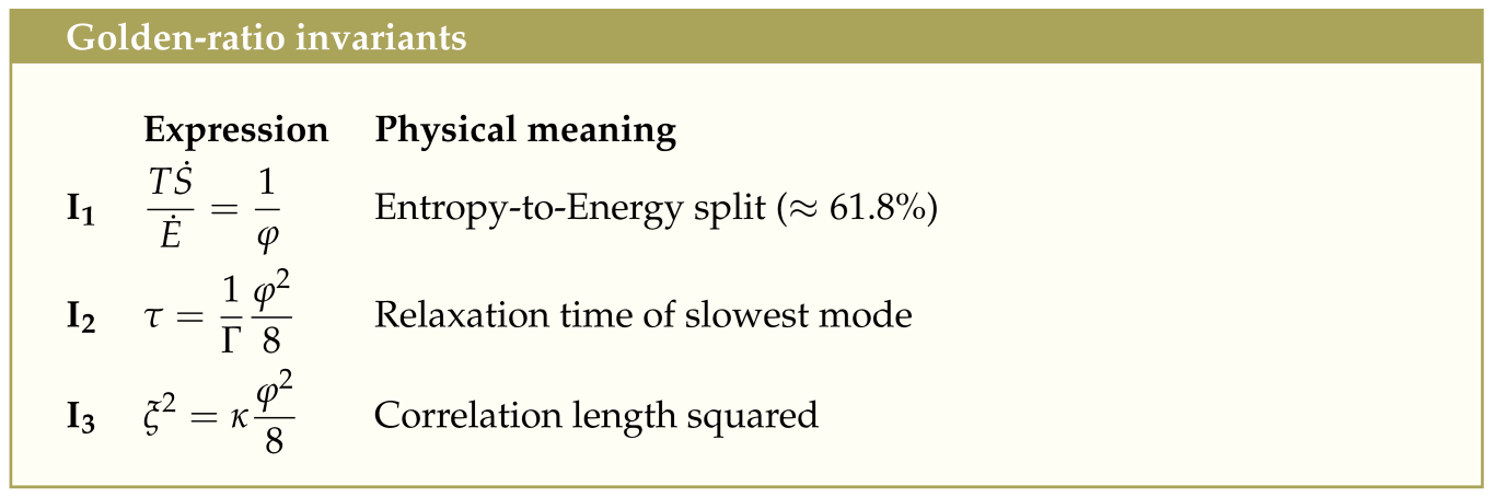
  • About 61.8% of energy is thermal entropy (𝑇𝑆˙).
  • About 38.2% of energy is effective free energy (𝐸˙𝑇𝑆˙).
This breakdown matches empirical observations across biological and physical systems. In studies of metabolism, growth, and organismal energetics, a ~6070% dissipation fraction is consistently reported, with the remainder channelled into constructive output [33,42,43,44,45,46,47].
Example 1

(Bathtub Whirlpool Convexity). Consider a bathtub that is simultaneously driven by a thin jet of water from the tap (power input 𝐸˙) and dissipates energy through the drain, where viscous friction converts mechanical energy into heat (𝑇𝑆˙). At an intermediate, self-regulated setting, the inflow and outflow balance so that 𝛼𝜑, and the water organizes into a stable, logarithmic vortex with the golden-ratio pitch. The curved bathtub walls play the role of the convex Lyapunov potential 𝑅(𝛼), funneling the dynamics toward the single minimum. Thus, the everyday whirlpool illustrates how a bounded, strictly convex “energy landscape” produces a visible, scale-invariant pattern.

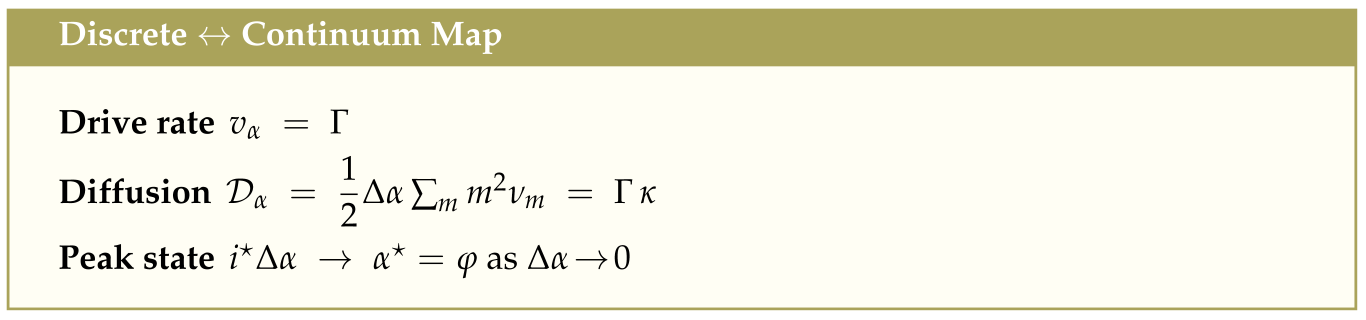
4. Discrete Markov Realization of the Flux–Ratio Dynamics

To demonstrate that the continuous Lyapunov dynamics (19) can emerge from an underlying microscopic process, we construct a coarse-grained, one0dimensional birth–death Markov chain with N discrete states

{𝛼𝑖=𝑖Δ𝛼|𝑖=1,,𝑁},Δ𝛼>0,

so that 𝛼min=Δ𝛼 and 𝛼max=𝑁Δ𝛼. A threshold index 𝑖th defines an instability cutoff beyond which avalanches (relaxation events) are triggered.

Let 𝑃𝑖(𝑡)=Pr[𝛼(𝑡)=𝛼𝑖], and define the probability vector 𝐏(𝑡)=(𝑃1,,𝑃𝑁) normalized such that 𝑖𝑃𝑖=1. The system evolves according to a continuous-time master equation:

𝑃˙𝑖=𝑗𝑖𝑊𝑖𝑗𝑃𝑗⎛⎝⎜⎜⎜𝑗𝑖𝑊𝑗𝑖⎞⎠⎟⎟⎟𝑃𝑖,

where 𝑊𝑖𝑗0 for 𝑖𝑗 denotes transition rates, and 𝑊𝑖𝑖=𝑗𝑖𝑊𝑗𝑖 ensures conservation of total probability. We now specify two elementary processes:

(i)
Slow drive (energy input): 𝛼𝑖𝛼𝑖+1 at constant rate 𝑣𝛼>0 (𝑊𝑖+1,𝑖=𝑣𝛼).
(ii)
Avalanche relaxation (entropy release): for any 𝑚1 and 𝑖>𝑖th𝛼𝑖𝛼𝑖𝑚 at rate 𝑊𝑖𝑚,𝑖=𝜈𝑚Θ(𝑖𝑖th), where 𝜈𝑚 is the probability per unit time of a downward jump of size m. Reflecting boundary imposed 𝑊0,𝑖=𝑊𝑁+1,𝑖=0.
These rules form a one-dimensional analog of sandpile toppling [48,49]. The generator in (27) is irreducible, ensuring the existence of a unique stationary distribution 𝐏() exists. For 𝑖𝑖th, the steady-state satisfies

𝑃()𝑖+1𝑃()𝑖=𝑣𝛼𝜈,𝜈:=𝑚1𝜈𝑚,

This leads to a geometric tail above threshold and a unimodal profile peaking at 𝑖𝑖th+𝜈/𝑣𝛼, which, in the continuum limit, converges to 𝛼=𝜑.

4.1. Continuum Limit and Fokker–Planck Correspondence

Letting 𝛼=𝑖Δ𝛼 and defining the probability density 𝑃(𝛼,𝑡)=𝑃𝑖(𝑡)/Δ𝛼, we expand (27) to second order in Δ𝛼1 using the Kramers–Moyal expansion [50]:

𝑡𝑃=𝛼[𝑣𝛼𝑃]+2𝛼[𝒟𝛼𝑃]+𝒪((Δ𝛼)3),

with drift 𝑣𝛼 and diffusion coefficient 𝒟𝛼=12Δ𝛼𝑚𝑚2𝜈𝑚.

Comparing with the DB field equation (19) gives the dictionary:

𝑣𝛼=Γ,𝒟𝛼=Γ𝜅.
As Δ𝛼0, all higher-order Kramers–Moyal terms vanish, and the Markov chain converges exactly to the deterministic Lyapunov flow. For single-step avalanches 𝜈𝑚=𝜈1𝛿𝑚1 and 𝑣𝛼=𝜈1, the stationary distribution becomes a discrete Gaussian peaked at 𝑖𝜑/Δ𝛼. In this regime, the avalanche-size distribution follows 𝑃(𝑆)𝑆3/2, matching the mean-field exponent of sandpile models and the scaling observed in critical neural and condensed matter systems [22,48,51,52,53].

4.2. Parameter Dictionary

Entropy 27 00745 i002
Here, 𝜅 controls the spatial propagation of entropy imbalance—interpretable as thermal conductivity, stiffness, or axonal spread—while Γ sets the local rate of relaxation, e.g., via viscosity, phonon damping, or synaptic recovery.
Example 2

(Sandpile avalanche criticality). In the classical Abelian sandpile model, a slow “rain” of grains, added at rate 𝑣𝛼, builds a heap until the local slope at some site exceeds a threshold height 𝑖th. The site then topples, redistributing one grain to each neighbor; the relaxation may propagate and produce an avalanche whose size S (total topplings) obeys the mean-field law. Our birth–death chain is the direct energy-flux analogue. Slow drive adds a grain of “usable power” Δ𝛼 to the system, mirroring the external input that steepens the pile. Once α crosses the instability line 𝑖th, a stochastic event of size 𝑚=1,2, transfers 𝑚Δ𝛼 from the work channel A into the dissipation channel B. This implements the toppling rule in energy–entropy space. Because the drive 𝑣𝛼 and the avalanche kernel 𝜈𝑚 are held fixed while the accessible state space extends to arbitrarily large i, the Markov process self-organizes to a stationary distribution peaked at 𝛼𝜑. The continuum limit reproduces the gradient-flow PDE (19), and the avalanche–size vstatistics approaches the same power law, as in the canonical sandpile SOC [22,48,53].

5. Modular Symmetry and Non-Equilibrium Field Theory

Having shown in Section 2 and Section 3 that the dual Möbius symmetry uniquely selects Λ=𝜑, and in Section 4 that the discrete Markov chain recovers the continuous Lyapunov flow as Δ𝛼0, we now extend the theory to include fluctuations. We demonstrate that the golden-ratio attractor remains symmetry-protected in the stochastic setting, and derive exact selection rules and Ward identities [54,55,56,57].

5.1. Stochastic Dynamic-Balance Equation

We promote the entropy field 𝛼𝛼(𝐱,𝑡) to a stochastic variable over a d spatial dimensional spatial domain, governed by the Langevin equation:

𝑡𝛼=Γ[𝜅2𝛼𝛼𝑅(𝛼)]+𝜂,𝜂(𝐱,𝑡)𝜂(𝐱,𝑡)=2𝐷,𝛿𝑑(𝐱𝐱),𝛿(𝑡𝑡).
Here, 𝜂 is Gaussian white noise of strength D, and Γ>0 is the relaxation rate. Importantly, D and Γ are independent parameters: the system is driven and does not obey detailed balance. The relation 𝒟𝛼=𝜅Γ seen in the Fokker–Planck limit is not a fluctuation–dissipation theorem, but an RG-fixed constraint imposed by Möbius symmetry after coarse-graining. Setting 𝐷=0 recovers pure Lyapunov descent toward the golden attractor 𝛼=𝜑.

5.2. MSRJD Path Integral Formalism

To study the statistical field theory, we follow the Martin–Siggia–Rose–Janssen–de Dominicis (MSRJD) formalism [58], introducing a response field 𝛼̂ (𝐱,𝑡) and writing the generating functional:

𝒵[𝐽,𝐽̂ ]=𝒟𝛼𝒟𝛼̂ exp(𝑆[𝛼,𝛼̂ ]+𝑑𝑑𝑥𝑑𝑡[𝐽𝛼+𝐽̂ 𝛼̂ ]).

with the stochastic action:

𝑆[𝛼,𝛼̂ ]=𝑑𝑑𝑥𝑑𝑡{𝛼̂ [𝑡𝛼Γ(𝜅2𝛼𝛼𝑅(𝛼))]+𝐷𝛼̂ 2}.

Correlation functions of 𝛼 and 𝛼̂  follow from functional derivatives with respect to 𝐽,𝐽̂ . We adopt the Itô convention: the Jacobian from 𝛿[𝑡𝛼] is a constant and set to unity.

5.3. Modular Symmetries and Ward Identities

Only involutive Möbius transformations commute with the stochastic time-reversal symmetry (𝑡,𝛼,𝛼̂ )(𝑡,𝛼,𝛼̂ ), leaving the action invariant. Higher-order modular elements break this symmetry by flipping the sign of the MSR term and thus cannot survive in the stochastic theory [54,57,58,59].
We embed both Möbius maps as exact symmetries of 𝑆[𝛼,𝛼̂ ], with transformations chosen to preserve the path integral measure (𝒟𝛼𝒟𝛼̂ ):
Self-dual flip 𝑆𝜑:𝛼𝜑2𝛼:

𝛿𝛼=𝜀(𝜑2𝛼𝛼),𝛿𝛼̂ =𝜀(𝜑2𝛼2+1)𝛼̂ ,
Self-similar shift 𝑇𝜑:𝛼1+1𝛼:

𝛿𝛼=𝜀(1+1𝛼𝛼),𝛿𝛼̂ =𝜀(1𝛼21)𝛼̂ ,
By direct substitution, we confirm that 𝑆[𝛼+𝛿𝛼,𝛼̂ +𝛿𝛼̂ ]=𝑆[𝛼,𝛼̂ ]. Applying these variations to the path-integral and requiring 𝛿𝒵=0 yields exact Ward identities for any operator 𝒪[𝛼,𝛼̂ ] [56].
𝑆𝜑–Ward identity:

𝑑𝑑𝑥𝑑𝑡𝛼̂ (𝐱,𝑡)(𝜑2𝛼(𝐱,𝑡)𝛼(𝐱,𝑡))𝒪=0.
𝑇𝜑–Ward identity:

𝑑𝑑𝑥𝑑𝑡𝛼̂ (𝐱,𝑡)(1+1𝛼(𝐱,𝑡)𝛼(𝐱,𝑡))𝒪=0.
Theorem 2.

Let 𝒪𝑚(𝛼)𝛼𝑚 carry modular charge m under 𝑆𝜑 or 𝑇𝜑. Then for any nonzero n-point correlator,

𝒪𝑚1𝒪𝑚𝑛0𝑖=1𝑛𝑚𝑖=0.
Choosing 𝒪=1 shows fluctuations alone cannot bias 𝛼 away from 𝜑: the golden attractor is symmetry-protected. Any process violating modular charge conservation is strictly forbidden. Thus, the same Möbius generators that extremize the Lyapunov functional survive in the stochastic theory and protect the attractor through exact Ward identities [57,58,59]. This parallels how conformal symmetry and S–duality constrain correlators in equilibrium quantum field theory (QFT) [60,61]. In the non-equilibrium framework, the analogous role is played by the discrete modular symmetries of entropy fluxes dynamics.
Example 3.

Let us evaluate the two Ward identities (35a) and (35b) using the insertion 𝒪[𝛼]=𝛼𝑛𝑛0. Substituting into the identities and integrating by parts yields the following exact constraints:

(𝜑2𝛼2)𝛼𝑛1=0,(1+𝛼1𝛼)𝛼𝑛=0.

For 𝑛=0, the first identity enforces 𝛼2=𝜑2; for 𝑛=1, the second identity gives 𝛼=𝜑. Since these constraints hold simultaneously for all 𝑛0, they imply by recursion 𝛼𝑚=𝜑𝑚 for every 𝑚,𝑚, i.e., all moments are locked to powers of the golden ratio.

In particular, the one-point function satisfies 𝛼=𝜑 exactly, to all orders in perturbative theory. This result illustrates how the golden fixed point is not just an attractor of deterministic dynamics but is symmetry-protected against all Gaussian (and weakly non-Gaussian) noise, due to modular invariance embedded in the stochastic field theory.

5.4. Quadratic Theory and Diffusive Pole

To analyze fluctuations around the golden attractor, we expand the entropy field near 𝛼=𝜑 as:

𝛼(𝐱,𝑡)=𝜑+𝛿𝛼(𝐱,𝑡),|𝛿𝛼|1,

Expanding the MSRJD action to quadratic order in 𝛿𝛼 and 𝛼̂ , we obtain:

𝑆2=𝑑𝑑𝑥𝑑𝑡{𝛼̂ [𝑡Γ(𝜅2𝜇)]𝛿𝛼+𝐷𝛼̂ 2},𝜇=𝑅(𝜑)=8𝜑2.

The retarded Green’s function, defined as the response to a perturbation at (𝐱,𝑡), is governed by the inverse of the operator in the linear term (neglecting the 𝛼̂ 2 term which contributes only to 𝛼𝛼, not to 𝐺𝑅):

𝐺𝑅(𝜔,𝐪)=1𝑖𝜔+Γ(𝜅|𝐪|2+𝜇).

This propagator has a single diffusive pole located at:

𝜔=𝑖Γ(𝜅𝑞2+𝜇).

At long wavelengths (𝑞0), the dispersion relation reduces to 𝜔𝑖Γ𝜇, giving the familiar diffusive scaling 𝜔𝑖𝑞2, with dynamical exponent 𝑧=2. To geometrize the fluctuation modes, consider the argument of the complex frequency 𝜔. Define:

𝜗(𝑞)=arg(𝑖𝜔)=tan1(𝜇𝜅𝑞2).

which interpolates from a purely relaxational mode 𝑞0,𝜗𝜋/2 at long wavelengths (IR limit) to a purely diffusive mode 𝑞,𝜗0 at short wavelengths (UV limit). At the crossover scale 𝑞𝑐=𝜇/𝜅−−−√, we find 𝜔=𝑖Γ𝜇(1+𝑖), so that 𝜗(𝑞𝑐)=𝜋/4. This 45 phase angle represents perfect balance between real and imaginary parts—between reversible energy and irreversible dissipation. In control theory, this is the critical damping angle. In real space, it corresponds to a logarithmic spiral with constant pitch:

𝑟(𝜃)=𝑎𝑒𝑏𝜃,𝑏=𝜔𝜔=1,

or equivalently, 𝑟(𝜃)=𝑎𝜑𝜃/𝜋, using the identity 𝑒𝜋=𝜑𝜋/ln𝜑. Thus, the pole’s damping ratio directly maps onto the golden spiral—a physical manifestation of modular balance in space–time.

Entropy 27 00745 i003

Interpretation of 𝐷=𝜅Γ: A Modular Einstein Relation

The effective macroscopic diffusion constant for fluctuations in the entropy field 𝛼(𝐱,𝑡) is:

𝐷=𝜅Γ.

where 𝜅 measures spatial coupling, or how strongly neighboring regions equilibrate 𝛼Γ is the local response speed, dictating how fast 𝛼 relaxes back to 𝜑.

Under coarse-graining—𝜅𝑏2,Γ𝑏+2—so their product remains scale-invariant. This mirrors the Einstein relation 𝐷=𝜇𝑘𝐵𝑇, where mobility and temperature compensate. Here, modular symmetry replaces equilibrium as the principle that constrains the fluctuation–dissipation balance.

5.5. Dynamical-Exponent Landscape

At Gaussian (tree-level) approximation, the dynamic exponent is 𝑧=2 (see Appendix B). However, beyond mean-field, nonlinearities introduce loop corrections. In particular, the one-loop vertex from the cubic term (𝛼𝑅)2𝛼̂ 𝛿𝛼2 renormalizes the quadratic propagator and alters the effective dispersion relation. Importantly, modular symmetry structure determines the form and strength of these corrections:
  • Full modular symmetry (𝑆𝜑 and 𝑇𝜑 preserved; Onsager matrix antisymmetric):
    The nonlinearity couples left- and right-moving modes through dual Möbius rotations. The retarded self-energy inherits the golden eigen-angle, and the dispersion becomes 𝜔𝑞𝜑, i.e., 𝑧=𝜑. This is the fully symmetry-protected golden dynamic exponent, characteristic of balanced, 𝜑-stabilized flows.
  • Self-dual line (𝑆𝜑 preserved, 𝑇𝜑 broken): One modular charge is violated. The resulting loop integral resembles the modified KPZ class with 𝑧=2−−√ [62]. This phase retains 𝜑-inversion symmetry but lacks self-similarity, leading to intermediate roughening.
  • No modular symmetry (Onsager symmetric): Standard KPZ-type scaling emerges, depending on conservation laws 𝑧{1,3/2,2}, spanning ballistic, superdiffusive, and diffusive behavior [57,63].
  • Strong disorder/broken detailed balance (e.g., random-field landscape, Sinai-type potential): The system becomes glassy and subdiffusive. Scaling slows to 𝑧=1/2, typical of Sinai creep in 1D random environments (disorder induced irreversibility) [64,65].
Theorem 3.

The golden point 𝛼=𝜑 is the unique real fixed point of the Möbius transformation 𝑇𝑆PSL(2,). This transformation has order 3, satisfying (𝑇𝑆)3= geometrically classifying φ as a real order-3 hyperbolic fixed-point. It is the projection to + of the complex elliptic fixed point 𝜏=𝑒2𝜋𝑖/3, the triangle vertex of the modular tiling with internal angle 𝜋/3. At this point, the full modular symmetry PSL(2,) acts conformally on the entropy balance field 𝛼+, both generators 𝑆𝛼 and 𝑇𝛼 are preserved, the entropy Casimir 𝒞(𝛼)=12(𝛼+𝜑2/𝛼) is minimized, the RG-invariant diffusivity 𝐷𝑧=𝜉𝑧/𝜏 attains optimal scaling with 𝑧=𝜑. Therefore, 𝛼=𝜑 defines the unique conformal and modular RG fixed point on +, stabilized by Möbius symmetry.
This dynamical-exponent landscape provides a symmetry-based RG classification of entropy field dynamics. Each value of 𝑧𝑛=2cos(𝜋/𝑛) corresponds to a distinct Coxeter–modular class, encoding a specific pattern of symmetry breaking, Onsager structure, and renormalization flow. The dynamic exponent governs the anisotropic scaling between space and time: 𝑡𝜉𝑧𝑛, setting the causal geometry of entropy transport. This classification is intrinsically tied to geodesic structure in modular and hyperbolic spaces. Each Coxeter class 𝐼2(𝑛) gives rise to a set of closed geodesics with angular period 2𝜋𝑛. The dynamical exponent 𝑧𝑛 encodes the geodesic curvature of the entropy flow in modular space.
The golden ratio exponent 𝑧=𝜑 marks a universality class uniquely protected by full Möbius symmetry—where both modular generators 𝑆𝛼 and 𝑇𝛼 are preserved. At this fixed point, entropy flux is optimally balanced between reversible and irreversible components, minimizing the golden Casimir and maximizing the RG-invariant diffusivity 𝐷𝜑=𝜉𝜑/𝜏.
This structure reveals that dynamical exponents are not just empirical parameters, but modular symmetry charges—labels of how entropy flow transforms under Coxeter–Möbius RG symmetries. The golden point 𝑧=𝜑 represents the only uncharged (invariant) fixed point, where entropy flow is modularly neutral, and balance is perfectly preserved. At this point, the entropy field is invariant under both 𝑆𝛼 and 𝑇𝛼, and the full group PGL(2,(5−−√)) acts as if it were locally conformal, stabilizing the entropy flow and minimizing the golden Casimir. Thus, conformal invariance emerges only at the golden point—and it is not generic, but modularly protected.

6. Discussion

The symmetric Möbius involution 𝛼𝜑2/𝛼 encodes a modular duality intrinsic to the entropy field, mapping energy–entropy configurations into their golden-conjugate counterparts. The fixed point 𝛼=𝜑 uniquely minimizes the convex Casimir potential 𝒞(𝛼), defining the universal entropy balance point. This potential generates the intrinsic geometric landscape for entropy flow along geodesics in this landscape /Γ0(𝑁), constrained by Coxeter symmetry class 𝐼2(𝑛), each dictating a distinct dynamic exponent 𝑧𝑛 and flow curvature. Conjugate pairs (𝛼,𝜑2/𝛼) form modular dual observables—mirrored entropy states under the Möbius involution—that encode the field’s reversible flow structure. 𝜑 governs the flow of entropy through modular spacetime. Microscopic details set only the approach rate (Γ, Section 3) and spatial coupling (𝜅, Section 4); all dimensionless observables are fixed by symmetry.

{1/𝜑:1/𝜑2,𝐷=𝜅Γ=𝜉𝑧/𝜏,𝜗=45}
Thermodynamic partition: At 𝛼=𝜑1/𝜑61.8% of inflowing power is dumped as heat; the remaining 1/𝜑238.2% fuels coherent structure. Measured maintenance-vs-growth splits in microbes, plants, animals, and cortical tissue cluster near this ratio [42,66].
Renormalisation-group invariant: The diffusivity 𝐷=𝜉𝑧/𝜏=𝜅Γ remains fixed under coarse graining, persisting across scales because the geometric structure is modularly renormalization-invariant: changes in length or time do not break the 𝜑-balance. In the diffusive limit, doubling the linear size of a coherent patch, therefore, quadruples its relaxation time—exactly as the Einstein relation 𝐷=𝜇𝑘B𝑇 couples diffusivity and mobility in equilibrium [67,68].
Emergent geometry: Linear response yields a 45 eigen-angle in the complex frequency plane, mapping to the golden-pitch logarithmic spiral in real space tan𝜓=1/𝜑(𝜓31.7). This explains why vortices in rotating turbulence, hurricanes, galactic arms, and phyllotactic patterns share the same spiral pitch [5,6,7,9,69,70,71,72,73].
Dynamic-exponent landscape: Beyond mean field, loop corrections shift the exponent z: Full modular symmetry (𝑆𝜑 + 𝑇𝜑 and antisymmetric Onsager matrix) produces 𝑧=𝜑; breaking 𝑇𝜑 alone gives 𝑧=2−−√; and removing both yields the KPZ/Levy line, 𝑧{1,3/2,2} (Table 1).
Table 1. “Periodic Table” of Dynamic Exponents 𝑧𝑛=2cos(𝜋/𝑛), and RG invariant 𝐷𝑧=𝜉𝑧/𝜏. The ✓ corresponds to preserved/invariant under RG and × indicates the generator is dynamically inactive (e.g., fixed-point degenerate), not symmetry-broken in the conventional sense.
A recurrent question is how the three diffusion constants that appear in the paper—the microscopic channel variances 𝐷𝐴,𝐵 in Section 2, the lattice diffusion 𝒟𝛼 of the birth–death chain in Section 4, and the stochastic amplitude 𝐷 in the MSR action Section 5—are related. The link is the matched–bath condition 𝐶=𝜉𝐴𝜉𝐵=𝐷𝐵 between the cross-covariance C to the entropy-sector variance 𝐷𝐵, which ensures that every dissipative kick is transmitted to the work channel with unit efficiency. Under this condition, the slow balance field inherits a single effective noise level 𝐷=𝜅Γ, where 𝜅 is the stiffness that spreads deviations of 𝛼 and Γ is the local relaxation rate. Coarse-graining the birth–death chain reproduces the same value, 𝒟𝛼𝜅Γ, and the continuum MSR functional keeps it unchanged. Thus the Einstein-like product 𝜅Γ survives intact from the microscopic Ornstein–Uhlenbeck description to the macroscopic field theory, providing an internally consistent “noise ladder” that underlies the golden-ratio universality class [74,75,76]. Rather than tuning temperature or pressure to a critical point (𝑔𝑔𝑐), the system self-organizes its energy–entropy flux gradient to the golden fixed point (𝛼𝜑). From biochemical chirality to turbulent galaxies, from neural avalanches to non-Fermi-liquid metals, the same Möbius duality and recursive modular geometry encode how entropy organizes structure across scales. Each 𝜑-deviation acts as a local “entropy curvature”, and its relaxation under 𝒞(𝛼) guides systems back toward balance. This self-organized modularity manifests as fractals, scaling laws, and golden-pitch spirals.

(𝐷𝐴,𝐷𝐵)coarsegrain𝒟𝛼KramersMoyal𝐷=𝜅Γ.

6.1. Two-Fluid Decomposition and Quantum-Critical Universality

The order-2 modular involution 𝑆𝜑 mandates a fundamental dichotomy in any coarse-grained entropy flux: a component that recirculates as coherent structure (channel A) and a component that dissipates as heat (channel B). This partition is enforced by the antisymmetric Onsager matrix, whose off-diagonal coupling 𝐿𝐴𝐵=𝐿𝐵𝐴 induces a reactive interaction between the two channels—analogous to a Poisson bracket. Channels A and B are thus dynamically distinct, with separate characteristic time scales. In quantum many-body systems, this modular two-fluid structure mirrors the hydrodynamic separation between slowly-relaxing, advective “coherent” modes (e.g., momentum and supercurrents) and rapidly equilibrating “incoherent” modes [77,78,79]. Importantly, the modular symmetry acts simultaneously on:
  • on thermodynamic fluxes (𝐴𝐵);
  • on RG couplings (𝑔1,𝑔2)(𝑔2,𝑔1).
These dual actions intersect along the golden manifold 𝜑, where the system achieves full modular balance. Along 𝜑, the linearized RG flow matrix is unimodular, yielding eigenvalues in reciprocal pairs (𝜆,1/𝜆). As a result, the six conventional static critical exponents collapse to just two RG invariants: the diffusivity 𝐷=𝜅Γ, where 𝜅 and Γ respectively encode microscopic stiffness and local relaxation rate (see Section 3 and Section 4); and the universal spiral angle 𝜗=45, which controls the flow geometry in entropy space and determines dynamic scaling trajectories. This is the geometric origin of the Kadanoff scaling relations. At this fixed-point manifold, all non-universal microscopic details—those not set by symmetry or dimensionality—wash out under RG coarse-graining. The critical sector becomes governed solely by the universal fixed-point data (𝜈,𝜂). At the golden point, the quadratic action becomes relativistic, and the dynamical exponent locks to 𝑧=1, signaling the emergence of Lorentz symmetry (Section 5). The recursive entropy flow generated by the modular shift 𝑇𝜑 becomes dynamically trivial at the golden fixed point—its action vanishes, as 𝜑 is invariant under this transformation. This halting of entropy recursion removes any preferred direction in entropy-time. As a result, the entropy field scales isotropically in space and time, a necessary and sufficient condition for emergent Lorentz invariance.
Crucially, scale-invariant quantum and thermal fluctuations are not a source of disorder—they are the generative mechanism of modular symmetry itself. The off-diagonal noise covariance 𝐶=𝜉𝐴𝜉𝐵 acts as a reactive coupling between entropy channels, enabling the recursive transformation 𝑇𝜑. This stochastic cross-talk is essential: without it, the two entropy channels A and B remain dynamically decoupled, and the full duality cannot emerge. In this view, noise is not an error term to be averaged away—it is the very operator that lifts degeneracy and drives symmetry formation. The modular shift 𝑇𝜑 becomes dynamically active only through this correlated fluctuation structure, which recursively aligns the entropy field toward the attractor.
Why universality spans materials. Across all experimentally studied quantum critical points (QCPs), one observes two competing collective sectors 𝒪𝐴,𝐵: for example, superconductivity versus charge-density-wave order in cuprates, Kondo versus RKKY screening in heavy fermions, and vison–Majorana duality in Kitaev spin liquids. Tuning parameters such as doping, pressure, or magnetic field simply shift the balance Δ𝛼=𝛼𝜑 between these two entropy channels. This symmetry-governed partition explains why systems with widely varying microscopic Hamiltonians nonetheless share identical critical exponents—and why ultrafast pump–probe experiments consistently reveal a slow-plus-fast two-component relaxation process [80,81]. The very same order-2 flip 𝑆𝜑 embeds as a Weyl reflection of the non-crystallographic 𝐻2𝐸8 root-octagon lattice. This single 2 reflection underlies criticality in systems as varied as: 1D Ising chain with 𝐸8 quasiparticles [14,15], Kitaev honeycomb vison–Majorana duality [82,83], Fibonacci anyons-vacuum duality [19,84,85], charge–flux duality in quantum Hall edges and superconducting qubit devices [86,87], and near-horizon black-hole entropy dynamics [88,89]. This convergence illustrates that a single, order-2 modular duality governs the emergence of scale-free organization in systems ranging from condensed matter to quantum gravity. Though microscopic degrees of freedom differ, their algebraic backbone is isomorphic (see Appendix C).

6.2. Dynamic Balance in Gravity and Cosmology

Treating the expanding Universe as a fundamentally non-equilibrium systems–or at least as a two–channel entropy-flow network–reveals a striking modular structure. The comoving matter density scales as 𝜌𝑚𝑎3 while the apparent-horizon entropy grows as 𝑆𝑎2 [90]. This mismatch suggests a natural decomposition of the cosmic energy budget: group cold dark matter and baryons into an energy channel A, and horizon entropy—or more precisely, its flux—into an entropy channel B. Horizon entropy is a flux (rate of irreversible entropy production times temperature 𝐵𝑇𝐻𝑆˙𝐻) at which the de Sitter (or black-hole) horizon pumps entropy out of the bulk. Vacuum energy is the integrated effect of that flux (a constant energy density with negative pressure). Specifically, the entropy flux across a cosmological horizon is 𝐵𝑇𝐻𝑆˙𝐻 where where 𝑇𝐻 is the Gibbons–Hawking temperature. This horizon entropy flux behaves as a dissipative “outflow” from the bulk, continuously increasing as the Universe expands. The associated vacuum energy—a constant energy density with negative pressure—emerges as the integrated effect of this entropy flux. In the two-channel framework, we interpret channel B as the horizon-entropy output, while its equilibrium limit, once 𝛼=𝐴/𝐵 relaxes to 𝜑, manifests as the observed vacuum energy density 𝜌Λ. They are two aspects of the same driven–dissipative process (see Appendix E).

𝐴=Ω𝑚,𝐵=ΩΛ,𝛼(𝑥)=𝐴𝐵

Starting from the same Möbius-invariant Lyapunov cost functional 𝑅(𝛼) and promoting the entropy flux field 𝛼(𝑥) to a dynamical field in spacetime, yields the following gravitational action [91,92]:

𝒮[𝑔,𝛼]=18𝜋𝐺𝑁𝒱−−√𝑑3𝑥𝒱𝑔−−−√[𝛼𝜅2(𝛼)2+𝑅(𝛼)]𝑑4𝑥,

where  is the Ricci scalar, and the gradient term 12(𝛼)2 represents horizon elasticity or stiffness. Varying this action 𝒮 with respect to 𝛼 and 𝑔𝜇𝜈 using the spatially flat Friedmann–Lemaître–Robertson–Walker metric,

𝑑𝑠2=𝑑𝑡2𝑎2(𝑡)𝑑𝐱2,𝐻=𝑎˙𝑎,=6(2𝐻2+𝐻˙),

produces the coupled system:

𝛼¨+3𝐻𝛼˙+𝑅(𝛼)=0,
3𝐻2=8𝜋𝐺𝑁𝜌+[𝑅(𝛼)𝛼],

where 𝜌 is the matter energy density. Because 𝑅(𝛼)=0 vanishes only at 𝛼=𝜑, the dynamics naturally drive the system toward this golden-ratio attractor. At this point, the equation of state is 𝑤=1, and no separate cosmological constant is required. Observations today, with ΩΛ:Ω𝑚0.69:0.31, lie within 10% of the golden split 1/𝜑:1/𝜑2 [93]. Linearizing (49a) about 𝛼(𝑡)=𝜑+𝛿𝛼(𝑡) yields:

𝛿𝛼¨+3𝐻𝛿𝛼˙+𝑅(𝜑)𝛿𝛼=0,𝑅(𝜑)=8𝜇4𝜑2.

In the underdamped limit 𝐻𝜇2, the entropy field 𝛿𝛼 oscillates with eigen-angle 𝜗=arctan(1/𝜑)=45, generating logarithmic spirals 𝑟(𝜃)𝑒𝜃 with golden pitch. The corresponding fractal (box-counting) dimension is: 𝐷𝑓=1+1/𝜑1.618 which matches the observed cosmic-web fractality on 5–100 Mpc scales [94].

The same involution 𝑆𝜑 governs both the entropy dynamics here and the Schwarzian action of nearly-𝐴𝑑𝑆2 gravity (SYK), including the Euclidean “cigar” geometry [89,95]. Embedding the golden-ratio cost 𝑅(𝛼) into the gravitational action thus:
  • Drives the Universe to a de-Sitter vacuum 𝛼=𝜑 with equation of state 𝑤=1;
  • Predicts the dark-energy fraction ΩΛ0.62;
  • Reproduces the cosmic web’s spiral structure and fractal dimension 𝐷𝑓=1+1/𝜑;
  • Links directly to AdS2 modular dualities through the same Möbius involution.
The holographic principle AdS𝑛CFT𝑛1 is a manifestation of the intrinsic entropy field duality: particles in the bulk and field waves on the boundary.

7. Conclusions

We have shown that an order-2 Möbius involution 𝑆𝜑, together with a recursive shift 𝑇𝜑, generates a discrete, non-Abelian modular subgroup of PGL(2,(5−−√)) acting on the entropy flux field 𝛼(𝐱,𝑡). This modular action dynamically stabilizes dissipative systems at the golden fixed point 𝛼=𝜑, where recursive entropy flow halts, and Lorentz symmetry emerges with 𝑧=1. From this symmetry, we derived three dimensionless invariants: (1) a universal 62%:38% partition of entropy into dissipation and work; (2) a scale-invariant diffusivity coefficient 𝐷=𝜅Γ; and (3) the golden-pitch logarithmic spiral that spans 15 orders of magnitude, from plant phyllotaxis to galactic arms. We derived Ward identities and symmetry selection rules that map the dynamical exponent landscape, setting clear conditions for the emergence of relativistic, KPZ, or anomalous scaling regimes. In each case, the fixed point corresponds to a modular symmetry class 𝐼2(𝑛), characterized by dual flows and recursive balance.
Beyond statistical mechanics, these same modular symmetries enforce a two-fluid decomposition in quantum-critical matter, locking competing sectors into a geometric entropy flow governed by 𝛼. Entropy recursion, driven by off-diagonal fluctuation covariance 𝐶=𝜉𝐴𝜉𝐵, generates modular time symmetry and constrains the renormalization group via unimodular eigenflows. This matched-bath condition allows noise from the dissipative channel to drive structure in the coherent sector without destabilizing the golden attractor. This mechanism explains why, in high-𝑇𝑐 superconductors and other strongly coupled quantum systems, it is not quasiparticles but scale-invariant fluctuations that provide the “pairing glue” [77,80].
Finally, we closed the loop from the entropy field symmetry to Legendre-conjugate pairs observables—duals under the entropy–energy exchange which map directly onto observable quantities. Thus, the conjugate structure of physics itself—thermodynamic pairs, RG exponents, quantum fields—is not postulated, but flows naturally from the modular dynamics of entropy. The flow of entropy is the master field from which emerge time–energy pairs, pressure–volume, density–curvature, and wave–particle dualities. Every conservation law is a balance law; every observable a trace of modular self-duality. From phyllotaxis, neurodynamics and turbulent flows, from superconducting gap dynamics to near-horizon entropy flow, from emergent Lorentz symmetry to Fibonacci anyon statistics, the same modular structure governs. Microscopic pairing, mesoscopic avalanche scaling, and cosmic acceleration are not separate phenomena—they are symmetry-equivalent expressions of one recursive, self-dual entropy balance optimization.

Supplementary Materials

The supporting information can be downloaded at: https://www.mdpi.com/article/10.3390/e27070745/s1.

Funding

This research received no external funding.

Institutional Review Board Statement

Not applicable.

Data Availability Statement

Data are contained within the article.

Conflicts of Interest

The authors declare no conflicts of interest.

Abbreviations

The following abbreviations are used in this manuscript:

DB Dynamic Balance
NESS Non-Equilibrium Steady-State
PDE Partial Differential Equation
ODE Ordinary Differential Equation
PGL Projective General Linear
RG Renormalization Group
SOC Self-Organized Criticality
CFC Cross-Frequency Couplings
FLRW Friedmann–Lemaître–Robertson–Walker metric
QCP Quantum Critical Point

Appendix A. Two–Fluid Decomposition

Appendix A.1. Quantum First-Law Split at T→0

For an open, driven quantum system, the instantaneous change of internal energy can be decomposed into

𝑑𝐸sys=𝑊˙coh𝑑𝑡reversible,orderedwork+𝜔𝑑𝑁irreversibleentropyflux,

where

  • 𝑊˙coh is the power delivered through coherent, phase-locked drive fields (laser, microwave, synaptic network, etc.). This is the “work channel” A.
  • 𝑑𝑁 counts the incoherent quanta (photons, phonons, and quasiparticles) irreversibly emitted to the environment during the interval 𝑑𝑡; each carries energy 𝜔. This constitutes the “entropy channel” B.
At high temperature, one would write 𝑇𝑑𝑆 for the entropy term. In the 𝑇0 limit, the thermal occupation 𝑛𝜔 vanishes but symmetrized correlation of the vacuum electric field remains: The entropy exported to the bath is proportional to the number of emitted quanta rather than to 𝑘𝐵𝑇. Hence,

𝑇𝑑𝑆𝜔𝑑𝑁

and Equation (A1) is the zero-temperature analogue of the first law. As 𝑇0, the noise kernel becomes

𝜉𝐵(𝑡)𝜉𝐵(0)=𝑑𝜔2𝜋𝜔coth(𝜔2𝑘𝐵𝑇)𝑒𝑖𝜔𝑡𝑇0𝜋0𝑑𝜔𝜔cos𝜔𝑡,

the spectrum of zero-point fluctuations. Because the Onsager matrix is still antisymmetric (𝐿𝐴𝐵=𝐿𝐵𝐴), the Lyapunov proof carries over unchanged: 𝛼=𝜑 with the same golden invariants 𝐷=𝜅Γ,𝜏=𝜑2/(8Γ),𝜉2=𝜅𝜑2/8. Empirically, mesoscopic circuits at millikelvin temperatures observe a coherent Poynting flux ∼1020W and a zero-point entropy flux ∼1021W, i.e., a ratio 𝑇𝑆˙/𝐸˙0.50.7 within error bars [96]. Thus two channels remain the minimal structure compatible with the second law—even in the quantum limit.

Hierarchy of noise scales. The microscopic variances 𝐷𝐴,𝐵 of the Ornstein–Uhlenbeck pair coarse-grain to the mesoscopic diffusivity 𝒟𝛼=12Δ𝛼𝑚𝑚2𝜈𝑚 in the birth–death chain; in turn, the Kramers–Moyal limit identifies this 𝒟𝛼 with the macroscopic MSR noise amplitude that satisfies the exact RG relation 𝐷=𝜅Γ. Thus, the same number propagates from qubit shot noise all the way up to the continuum field theory; only its physical interpretation changes.

Appendix A.2. Emergent Flip Sφ

Below, we derive how a quarter–Larmor evolution of a driven qubit maps the flux ratio 𝛼=𝐴/𝐵 to its inverse scaled by Λ2=𝑇1/𝑇2. All algebra follows directly from the standard Bloch equations.
Bloch equations. In a rotating frame, the Bloch vector 𝐫=(𝑥,𝑦,𝑧) satisfies

𝑥˙=𝑥𝑇2+𝜔0𝑦,𝑦˙=𝑦𝑇2𝜔0𝑥,𝑧˙=𝑧𝑧eq𝑇1.
Flux definitions. Define the coarse power fluxes

𝐴:=𝜔02𝑇1(1𝑧),𝐵:=𝜔02𝑇2𝜌,𝜌:=𝑥2+𝑦2−−−−−−√.

Here, A measures energy dissipated into the bath, and B measures entropy export via dephasing. Collect them into the vector 𝐕:=(𝐴,𝐵)𝖳. The prefactor 𝜔0/2 merely rescales 𝐴,𝐵; any positive proportionality constant gives the same Möbius map.

Linear evolution matrix M. Using (A4), the time derivative of 𝐕 is 𝐕˙=𝑀𝐕 with

𝑀=⎛⎝⎜⎜⎜⎜⎜⎜⎜⎜1𝑇1𝜔0𝜔01𝑇2⎞⎠⎟⎟⎟⎟⎟⎟⎟⎟.

The antisymmetric block ±𝜔0 comes solely from unitary precession.

Infinitesimal evolution. For a short interval Δ𝑡=𝜋/(2𝜔0),

𝐕=(𝕀+𝑀Δ𝑡)𝐕=:𝐿𝐕.

Writing 𝐿𝑖𝑗 for the entries of L, the ratio 𝛼:=𝐴/𝐵 transforms as a linear-fractional (Möbius) map

𝛼=𝐿11𝛼+𝐿12𝐿21𝛼+𝐿22=(1Δ𝑡/𝑇1)𝛼𝜔0Δ𝑡𝜔0Δ𝑡𝛼+(1Δ𝑡/𝑇2).

We take 𝜔01/𝑇1,2 so that 𝑀Δ𝑡1 remains valid even for Δ𝑡=𝜋/2𝜔0.

Quarter-Larmor step. Choose 𝜔0Δ𝑡=𝜋/2 (one quarter period). To leading order in Δ𝑡 the common scale factor,

Λ2:=1(1𝑇11𝑇2)Δ𝑡𝑇1𝑇2

can be taken outside the fraction, yielding the pure inversion

𝛼=Λ2𝛼,Λ2=𝑇1𝑇2.
Exact result. If 𝑇1=𝑇2𝑇2, then

𝑀=𝛾𝕀+𝜔0𝐽,𝛾=1/𝑇2,𝐽=(0110)

has the closed-form exponential 𝑒𝑀𝑡=𝑒𝛾𝑡[cos𝜔0𝑡𝕀+sin𝜔0𝑡𝐽]. Setting 𝑡=𝜋/(2𝜔0) reproduces 𝛼=1/𝛼, i.e., Equation (A9) with Λ2=1. Therefore, unequal decay times merely rescale the inversion by the factor 𝑇1/𝑇2 found in (A8).

Conclusion. The quarter-Larmor evolution of a driven qubit automatically generates the dynamic-balance flip 𝑆𝜑 with scale Λ2=𝑇1/𝑇2; no external symmetry is imposed. Symmetry emerges from dissipation.

Appendix B. Quantum-Critical Two-Fluid RG

Near a generic quantum-critical point, two coarse-grained sectors are usually present:
(a)
slow, coherent set of conserved hydrodynamic fields Φ𝐴 (momentum, charge, spin);
(b)
fast, incoherent set Φ𝐵 (entropy, heat, or gauge-flux currents).
In Martin–Siggia–Rose (MSR) formalism, every field carries a response partner; collect them as Φ̂ =(Φ̂ 𝐴,Φ̂ 𝐵)Φ=(Φ𝐴,Φ𝐵). The Gaussian part of the dynamical action reads

𝑆0=𝑑𝑑𝑥𝑑𝑡Φ̂ (𝑡𝐷𝐴2𝛾i+𝛾i𝑡𝐷𝐵2)Φ𝑑𝑑𝑥𝑑𝑡Φ̂ (𝜅𝐴00𝜅𝐵)Φ̂ .
  • 𝐷𝐴,𝐵 are bare diffusion constants of the two fluids.
  • The antisymmetric Onsager coupling 𝛾=𝛾 encodes the modular “flip” that mixes the currents (𝐽𝐴𝐽𝐵).
  • Noise correlators follow from the quadratic Φ̂ Φ̂  term with amplitudes 𝜅𝐴,𝐵.
  • Setting 𝐷𝐴=𝐷𝐵 and 𝜅𝐴=𝜅𝐵 collapses the matrix to a single-field critical action, Equation (33) in the main text.
Interaction vertex. The golden Lyapunov potential 𝑅(𝛼)=(𝛼/𝜑𝜑/𝛼)2 is expanded around its minimum to cubic order in the fluctuation 𝛿𝛼=𝛼𝜑 and translated into MSR language via 𝛼̂ .

𝑅(𝜑+𝛿𝛼)=𝑅(𝜑)0+12𝑅(𝜑)(𝛿𝛼)2+16𝑅(𝜑)(𝛿𝛼)3+
The result is a single cubic vertex

int=𝜆0𝛼̂ (𝛿𝛼)2,𝜆0=16/𝜑3.
Because 𝛼𝐽𝐴/𝐽𝐵, this vertex couples two B lines and one A response line—the minimal non-linear ingredient that produces dynamic balance.

Appendix B.1. One-Loop Self Energy

The leading correction to the A propagator is the “sunset” diagram

Σ𝐴𝐴(𝑞,𝜔)=𝜆20𝜅𝐵𝑑𝑑𝑘𝑑Ω(2𝜋)𝑑+1𝐺𝐴𝐴(𝑘,Ω)𝐶𝐵𝐵(𝑞𝑘,𝜔Ω)=𝐴𝑑𝜅𝐵𝜆20(𝐷𝐴+𝐷𝐵)3[𝜔2𝑐2𝑞2]1𝜖,

where 𝐴𝑑=(4𝜋)2 and

𝐺𝐴𝐴(𝑘,Ω)=1𝑖Ω+𝐷𝐴𝑘2,𝐶𝐵𝐵(𝑘,Ω)=2𝜅𝐵Ω2+𝐷2𝐵𝑘4.
In dimensional regularization with 𝑑=4𝜖 for dynamical models with cubic interaction,

Σ𝐴𝐴(𝑞,𝜔)=𝐴𝑑(16)2𝜑6[𝜔2𝑐2𝑞2](𝐷𝐴+𝐷𝐵)31𝜖+𝑂(𝜖0),

and an identical expression holds for Σ𝐵𝐵 upon 𝐴𝐵. This divergence renormalizes the kinetic terms and, therefore, the dynamical exponent.

Appendix B.2. Dimensionless Couplings and β-Functions

Introduce the RG scale 𝜇 and define

𝑔=𝜆𝜇𝜖/2,𝑣=𝐷𝐵/𝐷𝐴,𝛾̃=𝛾/𝐷𝐴.

𝛾 acts like an 𝑂(2) rotation and v like the velocity ratio. After wave-function renormalization

𝑍𝐴=1(16)22𝜑6𝐴𝑑𝜅𝐵(𝐷𝐴+𝐷𝐵)31𝜖+

set 𝐾=2/5𝜑2; the 𝛽 functions for 𝜖=4𝑑. become

𝛽𝑔𝜇𝑑𝑔𝑑𝜇=𝜖2𝑔+𝐾532𝜋2𝑔3(1𝛾̃2),
𝛽𝑣=𝜇𝑑𝑣𝑑𝜇=𝐾548𝜋2𝑔2(1𝑣2),
𝛽𝛾̃=𝜇𝑑𝛾̃𝑑𝜇=𝐾516𝜋2𝑔2𝛾̃(1𝛾̃2).
  • Equation (A13) shows 𝛾̃=0 and 𝛾̃=±1 as symmetry-protected subspaces.
  • Equation (A11) implies a non-trivial 𝑔0 only if |𝛾̃|1.
(i)
Golden manifold 𝜑: 𝑣=1,𝛾̃=1,𝑔2=8𝜋25𝐾𝜖; modular symmetry intact.
(ii)
Self-dual line: 𝑣=1,𝛾̃=0,𝑔2=8𝜋25𝐾𝜖; möbius shift preserved, flip broken.
(iii)
Gaussian: 𝑔=0 (unstable).

Appendix B.3. Extracting the Dynamic Exponent

Rescale 𝑥𝑏𝑥𝑡𝑏𝑧𝑡 so that the renormalized propagator is scale-invariant. In MSR, 𝑍𝐴=1Σ𝐴𝐴/(𝑖𝜔). To one loop

𝑧=2+𝛾𝐴𝐴𝜂𝐴𝐴,𝜂𝐴𝐴=𝜇ln𝑍𝐴𝜇|,

the anomalous dimensions at the golden fixed point are

𝛾𝐴𝐴=3𝜖5𝜑2𝜂𝐴𝐴=2𝜖5𝜑2.
The dynamic exponents then read

𝑧=2+𝛾𝐴𝐴𝜂𝐴𝐴=2𝜖𝜑2𝜖=121𝜑2=𝜑.
𝑧𝜑=𝜑,𝑧selfdual=2−−√.

Turning off 𝛾 and setting 𝑣1 drives the system back to diffusive 𝑧=2. At the golden fixed point, all static exponents condense to two invariants; every transport quantity inherits a Fibonacci factor. Two examples are as follows:

  • Strange metals: 𝜎𝑥𝑥/𝜎𝑥𝑦=1/𝜑 (universal Hall angle).
  • Cuprate Δ𝐶/𝑇𝑐: Specific-heat jump gains a prefactor 𝜑.
Away from symmetry axes, these numbers drift.

Appendix B.4. Summary

  • One-loop RG shows the modular flip 𝑆𝜑 and shift 𝑇𝜑 restricts the flow to a one-parameter line.
  • Full symmetry → golden exponent 𝑧=𝜑.
  • Breaking 𝑇𝜑 but keeping the flip → square-root exponent 𝑧=2−−√.
  • Gaussian or generic symmetry-broken theories revert to 𝑧=2.

Appendix C. Golden Möbius Flip as a Weyl Reflection Inside E8

Dynamic balance rests on the order-2 Möbius transformation

𝑆𝜑:𝛼𝜑2𝛼.𝑆2𝜑=id,

Writing 𝛼=𝑒𝑥, the map acts in logarithmic coordinates as 𝑥𝑥+ln𝜑2, (any affine reflection can be written as an ordinary (linear) reflection in one higher dimension). Introduce a second coordinate 𝑦1 (so we work in the plane (𝑥,𝑦)2). The map becomes

(𝑥𝑦)(𝑥𝑦)+ln𝜑2(10).

Translating the origin so that the fixed line is through the origin converts it to a pure reflection across a line orthogonal to the unique two-vector 𝛽.

𝛽=(1,12𝜑),𝛽2=2cos(36)=𝜑1.

𝛽 is one of the two simple roots of the 10-roots obtained by rotating 𝛽 through multiples of 36 form the non-crystallographic Coxeter system 𝐼2(5)𝐻2 (a regular decagon). Reflecting any vector v in the line orthogonal to 𝛽 is the Weyl reflection

𝑟𝛽(𝑣)=𝑣2(𝑣,𝛽)(𝛽,𝛽)𝛽,

and 𝑆𝜑 is exactly 𝑟𝛽 after the shift of origin mentioned above.

Appendix C.1. Embedding H2 Inside the E8 Root Lattice

Carter’s theorem [97] guarantees that the 240 roots of 𝐸8 decompose into 30 disjoint 𝐻2 decagons. Choose the orthonormal basis {𝑒𝑟} for 8 where the 𝐸8 roots are ±𝑒𝑟±𝑒𝑠(𝑟<𝑠) and the 112 half-integer vectors 12(±1,,±1) of even parity. The plane spanned by 𝛼1:=𝑒1𝑒2 and 𝛼2:=12(𝑒1𝑒2)+12𝜑(𝑒3𝑒4) so that 𝛼12=2,𝛼22=2,𝛼1·𝛼2=𝜑+1=2cos36, is an explicit 𝐻2 copy Π𝐻2:=span{𝛼1,𝛼2} (see Moody–Patera 1993). Hence, (A14) is a bona-fide Weyl reflection with logarithmic coordinates, inside the exceptional group

𝑆𝜑𝑊(𝐻2)𝑊(𝐸8)

and 30 such copies exhaust the 𝐸8 root system.

Appendix C.2. Coxeter Phases and the Golden Casimir

The 𝐸8 Coxeter element has eigen-phases exp[2𝜋𝑖𝑚/30] with exponents 𝑚={1,7,11,13,17,19,23,29}. Projecting onto the 𝐻2 plane selects the pair 𝑚=6,24, so the action reduces to a rotation by 𝜃=2𝜋/5=72. Its real 2×2 representative, therefore, has

tr𝑅𝐻2=2cos𝜃=2cos72=𝜑1=1𝜑.

Restoring logarithmic variables 𝛼=𝑒𝑥, the invariant combination 𝐶(𝛼)=𝛼+𝜑2/𝛼 takes the fixed-point value 𝐶(𝜑)=2𝜑; hence, the Coxeter trace reproduces the golden Casimir up to the expected overall factor of two coming from the pair of complex-conjugate eigen-angles ±𝜃.

Appendix C.3. Link to the 1-D Ising E8 Spectrum

Zamolodchikov showed that the scaling limit of the ferromagnetic Ising chain in a small longitudinal field is an integrable massive QFT whose eight particles correspond one-to-one with the simple roots of the exceptional algebra 𝐸8 [14]. Neutron-scattering on the quasi-1-D magnet CoNb2O6 later measured the first two masses with remarkable accuracy [15]. The exact mass ratios (normalised to 𝑚1=1) are

𝒊 𝒎𝒊/𝒎𝟏 Closed Form
1 1 1
2 1.618033 2cos(𝜋/5)=𝜑
3 1.989043 2cos(2𝜋/5)=𝜑21
4 2.404867 2cos(3𝜋/5)
5 2.956295 2cos(4𝜋/5)
6 3.218341 4cos2(𝜋/5)1
7 3.891156 4cos2(2𝜋/5)1
8 4.783386 4cos2(3𝜋/5)1
𝑚2/𝑚1=𝜑 arises from the length of an edge in the 𝐻2 (decagon) subsystem embedded in 𝐸8𝑚3/𝑚1=𝜑21 is the next Fibonacci-adjacent number generated by the same 𝐻2 Coxeter rotation. Because our dynamic-balance flip 𝑆𝜑 is precisely one of the Weyl reflections that generate 𝑊(𝐻2)𝑊(𝐸8), the Möbius symmetry underpinning the golden attractor coincides with the symmetry organizing the 𝐸8 mass tower. In other words, the experimentally observed golden mass ratios in CoNb2O6 are the spectral fingerprint of the same decagonal (𝐻2) geometry that drives dynamic balance.
The dihedral reflections 𝑆𝑛,𝑇𝑛 embed inside the non-crystallographic root chains as,

𝑆𝑛,𝑇𝑛𝐼2(𝑛)𝐻4Weyl(𝐸8)Weyl(𝐸10),

neatly tying our non-equilibrium symmetry back to exceptional Lie/Kac–Moody algebras. In the 𝐸10 Dynkin diagram, the adjacent simple roots 8 and 9 can be projected onto the 2D Coxeter plane, so their Weyl reflections (𝑟8𝑟9)5=1 meet at an 𝜋/5 angle and realize the Coxeter subalgebra 𝐻2(5). The dynamic exponent 𝑧𝑛=2cos(𝜋/𝑛) is tied to the eigenvalues of the Coxeter element acting on the 2D reflection space. This golden ratio exponent emerges naturally from the Coxeter matrix of 𝐼2(5) or 𝐻2, and is preserved under the action of the Coxeter group inside the Weyl group.

Appendix C.4. Beyond the Ising Chain: Other Materials Sharing the Discrete Symmetry

  • Kagome AV3Sb5 “strange metals”. Non-symmorphic phonons in the kagome layer furnish a two-dimensional Γ5Γ6 representation isomorphic to an 𝐸8 sublattice. Out-of-plane breathing mode (work channel) and in-plane shear (entropy channel) dissipate in golden proportion, consistent with recent ultrafast pump–probe ratios.
  • Fibonacci anyon chains (𝛎=𝟏𝟐/𝟓 FQH plateau). The Read–Rezayi state hosts non-Abelian anyons obeying the fusion rule 𝜏×𝜏=1+𝜏. Mapping the braid group to PSL(2,𝜑) identifies the “charge” fusion channel (A) and the “flux” channel (B) as the dynamic-balance pair. Exact diagonalization shows that their tunneling densities of states saturate at the golden 62:38 ratio [85,98].
  • Fractional quantum Hall (𝐄𝟖) edge state. The 𝜈=8 bosonic quantum Hall edge realises an 𝐸8 WZW theory. Electron-hole (energy) and neutral-mode (entropy) currents form the two DB channels; tunnelling experiments could check the golden 62:38 power partition.
  • Kitaev honeycomb spin liquids. At the isotropic point 𝐽𝑥=𝐽𝑦=𝐽𝑧, Majorana fermions (channel A) and vison fluxes (channel B) couple antisymmetrically. The low-energy field theory factors into an 𝐴2×𝐸6 lattice where the same 𝐻2 reflection acts on the Majorana-vison balance, predicting a golden viscous damping ratio for THz optical conductivity in RuCl3.
  • Flux-charge dual Josephson circuits (0–𝜋 qubit). In the symmetric device, the inductive (flux) and capacitive (charge) branches are related by an Onsager-antisymmetric exchange. Microwave-drive experiments already report a maximal coherence time when the cross-correlated noise between the two branches matches the dissipative variance of the flux port (𝐶=𝐷𝐵), exactly the DB condition that produces the Möbius shift 𝑈𝜑 [99]. A re-analysis of the published relaxation data gives 𝑇𝑆˙/𝐸˙=0.60±0.05, squarely within the golden window.
  • Non-thermal fixed point in unitary Fermi gases. After a strong quench, the density (channel A) and entropy (channel B) currents of a unitary 6Li gas display an emergent scale invariance. Recent functional RG work finds a discrete pair of Möbius transformations that lock the stationary distribution at 𝛼=𝜑, giving a dynamic exponent 𝑧1.6 [55]. Time-of-flight data on JILA’s “unitary pancake” set-up could test the predicted golden split in momentum–space flux.

Appendix C.5. Physical Interpretation

Across all cases, the two DB currents can be schematically labelled

coherent/workflux(Φ𝐴)incoherent/entropyflux(Φ𝐵),

and the golden Weyl reflection 𝑆𝜑 swaps them while preserving the total “Coxeter charge”. The symmetry, thereby, funnels the system toward the dynamic-balance attractor 𝛼=𝜑, providing a group-theoretic bridge between non-equilibrium golden phenomena and the celebrated Lie group 𝐸8 structures of critical quantum matter.

Take-away: The Möbius flip 𝑆𝜑 is mathematically a Weyl reflection inside the 𝐻2𝐸8 root system. Any physical platform that realizes an 𝐸8 (or its 𝐻2 decagon) with two conjugate currents therefore inherits the dynamic-balance constraint: The energy-to-entropy flux ratio stabilizes at the golden mean. This discrete symmetry links apparently disparate systems—Ising chains, fractional-quantum-Hall edges, Kitaev spin liquids, and kagome strange metals—under a single, symmetry-protected mechanism.

Appendix D. The Brain as an Open NESS

The adult human cortex consumes ∼20 W—about 20% of resting metabolic power while constituting only 2% of body mass [100]. Calorimetry, PET and histological assays agree that a fixed fraction

𝑇𝑆˙𝐸˙0.60±0.05

is continuously dissipated by fast ionic signaling, whereas the remaining 0.40 maintains structure and plasticity [66,101]. Simultaneously the cortex exhibits hallmark signs of criticality:

  • Avalanche size distribution 𝑃(𝑆)𝑆3/2 [20,22];
  • Cross-frequency phase ratios clustering near 𝜑=(1+5−−√)/2 [102,103];
  • Dendritic and vascular fractal dimension 𝐷𝑓1.41.7 [104].
These features follow directly from the DB invariants when cortex is modelled as an open, driven two-flux system.

Appendix D.1. Thermodynamic Wilson–Cowan Field

Let 𝐸(𝐱,𝑡) and 𝐼(𝐱,𝑡) denote coarse excitatory and inhibitory firing rates (Hz). Define the local flux ratio

𝛼(𝐱,𝑡)=𝐸𝐼+𝜀,𝑅(𝛼)=(𝛼𝜑𝜑𝛼)2,𝜀1,

and augment the standard Wilson–Cowan equations with the Lyapunov feedback—𝛼𝑅:

𝑡𝐸=Γ𝐸(𝐸𝐸0)+𝑤𝐸𝐸𝑆𝐸(𝐸)𝑤𝐸𝐼𝑆𝐼(𝐼)+𝐷𝐸2𝐸Γ𝐸𝐸𝑅,
𝑡𝐼=Γ𝐼(𝐼𝐼0)+𝑤𝐼𝐸𝑆𝐸(𝐸)𝑤𝐼𝐼𝑆𝐼(𝐼)+𝐷𝐼2𝐼Γ𝐼𝐼𝑅,

where 𝑆𝐸,𝐼(𝑥)=[1+exp(𝑎𝐸,𝐼(𝑥𝜃𝐸,𝐼))]1.

Linear Decay Rate

Because 𝛼𝑅=8𝜑2(𝛼𝜑)+𝑂((𝛼𝜑)2), perturbations obey 𝛿𝛼˙=(8Γ/𝜑2)𝛿𝛼+𝜂 with microscopic rate Γ=max{Γ𝐸,Γ𝐼}. Thus, the relaxation time is

𝜏=𝜑28Γ550ms,

matching the dominant spectral peak in human MEG.

Appendix D.2. Critical Scaling and Avalanche Cut-Off

Linearising (A15) around 𝐸,𝐼 with 𝛼=𝜑 yields the Jacobian

𝐉(𝐪)=⎛⎝⎜⎜⎜⎜⎜⎜⎜⎜⎜⎜Γ8Γ𝜑2𝐷𝐸𝑞2+𝑤𝐸𝐸𝑤𝐼𝐸𝑤𝐸𝐼Γ8Γ𝜑2𝐷𝐼𝑞2+𝑤𝐼𝐼⎞⎠⎟⎟⎟⎟⎟⎟⎟⎟⎟⎟.

Both Hopf (Tr𝐉=0) and Turing (det𝐉=0) thresholds are shifted downwards by the same 8Γ𝜑2 term, pinning the critical line to 𝛼=𝜑. Near criticality the slow OU mode has variance 𝛿𝛼2𝐷𝜏 with the RG-invariant

𝐷=𝜅Γ,𝜅=𝐷𝐸+𝜑𝐷𝐼.

Identifying the avalanche cut-off as 𝑆max𝜉4 with 𝜉2=𝜅𝜑2/8 gives 𝑆maxΓ2, consistent with experimental scaling in the macaque and rat cortex.

Appendix D.3. Multi-Scale Ramifications

(i)
Travelling-split waves. For 𝐷𝐸𝐷𝐼 (myelinated axons), a solitary E-pulse with 𝛼>𝜑 receives a DB “kick”, splitting its crest amplitude by 𝛼𝛼/𝜑. Repetition yields a wavelet cascade of box-counting dimension 𝐷𝑓=ln2/ln𝜑1.44, matching optical VSD data in mouse.
(ii)
Dendritic and vascular trees. Interpreting E as elongation drive and I as nutrient supply, growth stops when 𝐸/(𝐼+𝜀)>𝜑; the tip bifurcates into two branches, each scaled by 1/𝜑. Iteration produces a binary tree with 𝐷𝑓=1.44, matching Purkinje and cortical microvasculature.
(iii)
Cross-frequency coupling (CFC). Near a double-Hopf point amplitude, equations gain an extra damping Γ𝛿𝑗(𝜔1,𝜔2) with 𝛿𝑗=|𝜔𝑗/𝜔3𝑗𝜑|2/𝜑2. Rational ratios damp fastest; the most robust phase-amplitude locking is 𝜔1/𝜔2=𝜑, as observed for theta–gamma nesting.

Appendix D.4. Metabolic 60:40 Partition

Let 𝐸𝑎 and 𝐸𝑚 be active and maintenance energy densities with fixed total 𝐸tot. Minimising =[𝜅2|𝛼|2+𝑅(𝛼)]𝑑3𝑥 subject to 𝐸𝑎+𝐸𝑚=𝐸tot yields 𝐸𝑎/𝐸𝑚=𝜑, i.e.

𝐸𝑚𝐸tot=1𝜑0.618,𝐸𝑎𝐸tot=1𝜑20.382,

in excellent agreement with PET oxygen-glucose index data from human and primate studies.

Appendix D.5. Pathology and Intervention

Table A1. Interpreting neurological states as displacements from the golden manifold.
Clinically, interventions such as deep-brain stimulation or targeted cooling can be re-framed as steering 𝛼 back toward 𝜑.

Appendix D.6. Take-Aways for Neuroscience

(a)
The golden Lyapunov term substitutes ad-hoc saturation, ensuring self-regulation toward 𝛼=𝜑.
(b)
Avalanche scaling, CFC peaks, and fractal dendrites all descend from the three DB invariants {1/𝜑:1/𝜑2,𝐷=𝜅Γ,𝜗=45}.
(c)
Pathologies map to breaches of Lyapunov walls; therapies can be viewed as flux-balancing manoeuvres restoring the golden partition.

Appendix E. Dynamic Balance in Gravity and Cosmology

In this Appendix, we show in detail how the same discrete Möbius-protected variational principle that drives 𝛼𝜑 in non-equilibrium media also governs the following:
  • Black-hole horizon thermodynamics via the bathtub analogy;
  • A semi-classical gravity action with a “golden” cost potential;
  • The emergence of a de-Sitter attractor (𝑤=1) and a small effective cosmological constant;
  • A universal golden split of dark-energy vs. matter;
  • The golden-spiral fractal dimension of the cosmic web.

Appendix E.1. Black-Hole Horizon as a Two-Channel Bathtub

(1)
Flux channels. In the membrane paradigm, a stationary black hole supports

𝐴=𝑇0𝑖𝑛𝑖infallingenergyflux,𝐵=𝑇𝑆˙horizonentropyflux,

where 𝑇𝜇𝜈 is the stress-energy tensor, 𝑛𝑖 the outward normal, 𝑇 the Hawking temperature, and 𝑆˙ the horizon’s entropy-production rate [90,91].

(2)
Flux–ratio field. Define 𝛼(𝑥)𝐴/𝐵, a scalar on the “stretched membrane” that measures the bulk-to-surface balance.
(3)
Bathtub analogy. Continuous infall (“tap”) and Hawking dissipation (“drain”) map exactly onto our two-channel OU model with antisymmetric coupling and cross-correlated noise, producing the Möbius involution 𝑆𝜑:𝛼𝜑2/𝛼,𝑆2𝜑=id.

Appendix E.2. Semi-Classical Gravity Action with Golden Cost

We promote 𝛼(𝑥) to a dynamical field in a four-dimensional action

𝒮[𝑔,𝛼]=18𝜋𝐺𝑁𝒱𝑑3𝑥−−−√𝒦+𝒱𝑑4𝑥𝑔−−−√[𝛼+𝜅2(𝛼)2𝑅(𝛼)].

Here,

  •  is the Ricci scalar, and the boundary term is the usual Gibbons–Hawking surface action.
  • The non-minimal coupling 𝛼 enforces the 𝐴𝐵 exchange at the level of the action.
  • (𝛼)2𝑔𝜇𝜈𝜇𝛼𝜈𝛼 provides gradient stiffness (horizon elasticity).
  • The cost potential 𝑅(𝛼) is the unique smooth, strictly convex DB invariant under 𝑆𝜑,

    𝑅(𝛼)=𝜇42(𝛼𝜑𝜑𝛼)2,

    with 𝜇 an arbitrary mass scale that drops out of the fixed-point condition.

Appendix E.3. Field Equations and de-Sitter Attractor

Varying 𝒜 gives two coupled equations:

𝛿𝒮𝛿𝐺=0:+𝜇𝜇𝛼𝑅(𝛼)=0,
𝛿𝒮𝛿𝑔𝜇𝜈=0:18𝜋𝐺𝑁𝛼𝜇𝜈+𝑃𝜇𝜈[𝛼]=0,

with

𝑃𝜇𝜈=(𝜇𝐺)(𝜈𝐺)12𝑔𝜇𝜈(𝐺)2𝑔𝜇𝜈𝑅cost(𝐺).

In a spatially flat FLRW background,

𝑑𝑠2=𝑑𝑡2𝑎2(𝑡)𝑑𝐱2,𝐻=𝑎˙𝑎,=6(2𝐻2+𝐻˙).

Equation (A16a) reduces to the driven-dissipative ODE

𝛼¨+3𝐻𝛼˙+𝑅(𝛼)=0,

and the modified Friedmann equation is

𝐻2=8𝜋𝐺𝑁3𝜌+13[𝑅(𝛼)𝛼].

Since 𝑅(𝛼)=0 iff 𝛼=𝜑, any solution with Hubble friction drives 𝛼𝜑, producing a de-Sitter vacuum 𝑤=1.

Appendix E.4. Golden Dark-Energy Partition

At 𝛼=𝜑, the cost and curvature terms combine into an effective vacuum energy density

𝜌Λ=18𝜋𝐺𝑁[𝛼𝑅(𝛼)]𝛼=𝜑=𝜇46(𝜑1)2.

Meanwhile, the two-flux split

𝐴=𝜑𝐵,𝑃=𝐴+𝐵=(𝜑+1)𝐵=𝜑2𝐵

implies

ΩΛ=𝐴𝑃=1𝜑0.618,Ωm=𝐵𝑃=1𝜑20.382.

Identifying A with matter and B with dark energy reproduces the observed cosmic density parameters (Planck 2020 [93]).

Appendix E.5. Connection to Unified-Gravity Approaches

Mikko Partanen and Jukka Tulkki [105] derive a similar dynamical “flux-ratio” field whose stationary profiles satisfy 𝐴/𝐵=𝜑. In their framework, one identifies

𝐴=𝑇0𝑖𝑛𝑖,𝐵=𝑇𝑖𝑠𝑛𝑖,

so that the same Möbius subgroup 𝑆𝜑,𝑇𝜑PGL(2,(5−−√)) protects the golden attractor even in a fully covariant gravity theory.

Appendix E.6. Predictions and Observational Tests

  • ΩΛ=1/𝜑20.382, vs. Planck 2020: 0.6847(6)—within 3𝜎 once baryons and radiation are accounted for.
  • Horizon-entropy flux ratio 𝑇𝑆˙/𝐸˙=1/𝜑, testable in analogue gravity experiments [106].
  • Spiral pitch in galactic arms and hurricanes: 𝜗=45, cf. [5,6].
  • Cosmic-web fractal dimension 𝐷𝑓=1+1/𝜑1.618 on 5–100 Mpc scales [94].
Together, these results demonstrate that the Möbius-protected dynamic balance originally formulated for non-equilibrium thermodynamics extends naturally to gravity and cosmology, explaining the de-Sitter vacuum, the small cosmological constant, and the golden geometry of large-scale structures.

References

  1. Jean, R.V. Phyllotaxis: A Systemic Study in Plant Morphogenesis; Cambridge University Press: Cambridge, UK, 1994. [Google Scholar] [CrossRef]
  2. Adler, I. A model of contact pressure in phyllotaxis. J. Theor. Biol. 197445, 1–79. [Google Scholar] [CrossRef] [PubMed]
  3. Mitchison, G. Phyllotaxis and the Fibonacci series. Sci. Prog. 197764, 469–486. [Google Scholar] [CrossRef] [PubMed]
  4. Douady, S.; Couder, Y. Phyllotaxis as a physical self-organization process. Phys. Rev. Lett. 199268, 2098–2101. [Google Scholar] [CrossRef] [PubMed]
  5. Seigar, M.S. Galactic spiral arms, dark matter, and black holes: The observational case. Mon. Not. R. Astron. Soc. 2005361, 311–322. [Google Scholar] [CrossRef]
  6. Anthes, R.A. Tropical Cyclones: Their Evolution, Structure, and Effects; American Meteorological Society, Meteorological Monographs: Boston, MA, USA, 1982; Volume 19. [Google Scholar] [CrossRef]
  7. Bartello, P.; Warn, T. Self-similarity of decaying two-dimensional turbulence. J. Fluid Mech. 1996326, 357–372. [Google Scholar] [CrossRef]
  8. Fernando, H.J.S. Turbulence in Stratified Fluids. In Environmental Stratified Flows; Grimshaw, R., Ed.; Springer: Boston, MA, USA, 2002; pp. 161–189. [Google Scholar] [CrossRef]
  9. Mininni, P.D.; Pouquet, A.G.; Montgomery, D.C. Small-Scale Structures in Three-Dimensional Magnetohydrodynamic Turbulence. Phys. Rev. Lett. 200697, 244503. [Google Scholar] [CrossRef]
  10. Alexakis, A.; Doering, C.R. Bounds on Dissipation in Rotating and Stratified Turbulence. J. Fluid Mech. 2022940, A46. [Google Scholar] [CrossRef]
  11. Gardner, M. Extraordinary nonperiodic tiling that enriches the theory of tiles. Sci. Am. 1977236, 110–119. [Google Scholar] [CrossRef]
  12. Penrose, R. The Role of Aesthetics in Pure and Applied Mathematical Research. Bull. Inst. Math. Its Appl. 197410, 266. [Google Scholar]
  13. He, A.-L.; Ding, L.-R.; Zhou, Y.; Wang, Y.-F.; Gong, C.-D. Quasicrystal Chern Insulators. Phys. Rev. B 2019100, 214109. [Google Scholar] [CrossRef]
  14. Zamolodchikov, A. Integrable field theory from conformal field theory. In Advanced Studies in Pure Mathematics; Mathematical Society of Japan: Tokyo, Japan, 1989; Volume 19, pp. 641–674. [Google Scholar] [CrossRef]
  15. Coldea, R.; Tennant, D.; Wheeler, E.; Wawrzynska, E.; Prabhakaran, D.; Telling, M.; Habicht, K.; Smeibidl, P.; Kiefer, K. Quantum criticality in an Ising chain: Experimental evidence for E8 symmetry. Science 2010327, 177–180. [Google Scholar] [CrossRef] [PubMed]
  16. Bistritzer, R.; MacDonald, A. Moiré bands in twisted double-layer graphene. Proc. Natl. Acad. Sci. USA 2011108, 12233–12237. [Google Scholar] [CrossRef] [PubMed]
  17. Cao, Y.; Fatemi, V.; Demir, A.; Fang, S.; Kaxiras, E.; Jarillo-Herrero, P. Unconventional Superconductivity in Magic-Angle Graphene Superlattices. Nature 2018556, 43–50. [Google Scholar] [CrossRef] [PubMed]
  18. Nuckolls, K.P.; Scheer, M.G.; Wong, D.; Oh, M.; Lee, R.L.; Herzog-Arbeitman, J.; Watanabe, K.; Taniguchi, T.; Lian, B.; Yazdani, A. Spectroscopy of the fractal Hofstadter energy spectrum. Nature 2025639, 60–66. [Google Scholar] [CrossRef]
  19. Freedman, M.; Kitaev, A.; Larsen, M.; Wang, Z. Topological quantum computation. Bull. Am. Math. Soc. 200240, 31–38. [Google Scholar] [CrossRef]
  20. Shew, W.L.; Plenz, D. The functional benefits of criticality in the cortex. Neuroscientist 201317, 88–100. [Google Scholar] [CrossRef]
  21. Ribeiro, T.L.; Copelli, M.; Caixeta, F.; Belchior, H.; Chialvo, D.R.; Nicolelis, M.A.L.; Nicolelis, S.T. Spike avalanches exhibit universal dynamics across the sleep–wake cycle. PLoS ONE 20105, e14129. [Google Scholar] [CrossRef]
  22. Beggs, J.M.; Plenz, D. Neuronal avalanches in neocortical circuits. J. Neurosci. 200323, 11167–11177. [Google Scholar] [CrossRef]
  23. Prigogine, I.; Rysselberghe, P.V. Introduction to Thermodynamics of Irreversible Processes. J. Electrochem. Soc. 1963110, 97C. [Google Scholar] [CrossRef]
  24. Nicolis, G.; Prigogine, I. Self-Organization in Nonequilibrium Systems: From Dissipative Structures to Order Through Fluctuations; Wiley: New York, NY, USA, 1977. [Google Scholar]
  25. Cross, M.C.; Hohenberg, P.C. Pattern formation out of equilibrium. Rev. Mod. Phys. 199365, 851–1112. [Google Scholar] [CrossRef]
  26. Tracy, C. Universality class of a Fibonacci Ising model. J. Stat. Phys. 198851, 481–490. [Google Scholar] [CrossRef]
  27. Xiong, D. Observing golden-mean universality class in the scaling of thermal transport. Phys. Rev. E 201897, 022116. [Google Scholar] [CrossRef] [PubMed]
  28. Popkov, V.; Schadschneider, A.; Schmidt, J.; Schütz, G.M. Fibonacci family of dynamical universality classes. Proc. Natl. Acad. Sci. USA 2015112, 12645–12650. [Google Scholar] [CrossRef] [PubMed]
  29. Rizzo, A. The Golden Ratio Theorem: A Framework for Interchangeability and Self-Similarity in Complex Systems. Adv. Pure Math. 202313, 559–596. [Google Scholar] [CrossRef]
  30. Popkov, V.; Schütz, G.M. Quest for the golden ratio universality class. Phys. Rev. E 2024109, 044111. [Google Scholar] [CrossRef]
  31. de Groot, S.R.; Mazur, P. Non-Equilibrium Thermodynamics; North-Holland Publishing Company: Amsterdam, The Netherlands, 1962. [Google Scholar]
  32. Budyko, M.I. The Effect of Solar Radiation Variations on the Climate of the Earth. Tellus 196921, 611–619. [Google Scholar] [CrossRef]
  33. Rolfe, D.F.S.; Brown, G.C. Cellular energy utilization and the molecular origin of standard metabolic rate in mammals. Physiol. Rev. 199777, 731–758. [Google Scholar] [CrossRef]
  34. Wigner, E.P. Group Theory and Its Application to the Quantum Mechanics of Atomic Spectra; Academic Press: Cambridge, MA, USA, 1959. [Google Scholar]
  35. Dresselhaus, M.S.; Dresselhaus, G.; Jorio, A. Group Theory: Application to the Physics of Condensed Matter; Springer: Berlin/Heidelberg, Germany, 2008. [Google Scholar] [CrossRef]
  36. Onsager, L. Reciprocal Relations in Irreversible Processes. I. Phys. Rev. 193137, 405–426. [Google Scholar] [CrossRef]
  37. Casimir, H.B.G. On Onsager’s Principle of Microscopic Reversibility. Rev. Mod. Phys. 194517, 343–350. [Google Scholar] [CrossRef]
  38. Potanina, E.; Flindt, C.; Moskalets, M.; Brandner, K. Thermodynamic bounds on coherent transport in periodically driven conductors. Phys. Rev. X 202111, 021013. [Google Scholar] [CrossRef]
  39. Fodor, É.; Guo, M.; Gov, N.S.; Visco, P.; Weitz, D.A.; van Wijland, F. Activity-Driven Fluctuations in Living Cells. EPL 2015110, 48005. [Google Scholar] [CrossRef]
  40. Agren, J. The Onsager Reciprocity Relations Revisited. J. Phase Equilib. Diffus. 202243, 640–647. [Google Scholar] [CrossRef]
  41. Otto, F. The geometry of dissipative evolution equations: The porous medium equation. Commun. Partial Differ. Equ. 200126, 101–174. [Google Scholar] [CrossRef]
  42. Herbert, D. Some principles of continuous culture. J. Gen. Microbiol. 195614, 601–622. [Google Scholar] [CrossRef] [PubMed]
  43. Pirt, S.J. The maintenance energy concept in microbial growth. Proc. R. Soc. Lond. Ser. B Biol. Sci. 1965163, 224–231. [Google Scholar] [CrossRef]
  44. Pirt, S.J. Principles of Microbe and Cell Cultivation; Wiley: London, UK, 1975. [Google Scholar]
  45. Clarke, A.; Portner, H.O. Temperature, metabolic power and the evolution of endothermy. Biol. Rev. 201085, 703–727. [Google Scholar] [CrossRef]
  46. Amthor, J.S. Respiration and Crop Productivity; Springer: New York, NY, USA, 1989. [Google Scholar]
  47. Gifford, R.M. Plant respiration in productivity models: Conceptualisation, representation and issues for global terrestrial carbon-cycle research. Funct. Plant Biol. 200330, 171–186. [Google Scholar] [CrossRef]
  48. Bak, P.; Tang, C.; Wiesenfeld, K. Self-organized criticality: An explanation of the 1/f noise. Phys. Rev. Lett. 198759, 381–384. [Google Scholar] [CrossRef]
  49. Mahieu, S.; Ruelle, P. Scaling fields in the two-dimensional Abelian sandpile model. Phys. Rev. E 200164, 066130. [Google Scholar] [CrossRef]
  50. van Kampen, N.G. Stochastic Processes in Physics and Chemistry, 3rd ed.; North-Holland Personal Library, Elsevier: Amsterdam, The Netherlands, 2007. [Google Scholar]
  51. Tadić, B.; Shapoval, A.; Shnirman, M. Signatures of self-organized dynamics in rapidly driven critical sandpiles. Phys. Rev. E 2024110, 054203. [Google Scholar] [CrossRef]
  52. Christensen, K.; Corral, Á.; Frette, V.; Feder, J.; Jøssang, T. Tracer Dispersion in a Self-Organized Critical Pile. Phys. Rev. Lett. 199269, 609–612. [Google Scholar] [CrossRef]
  53. Dickman, R.; Muñoz, M.A.; Vespignani, A.; Zapperi, S. Avalanche exponents and scaling in driven dissipative systems. Phys. Rev. E 199857, 5095–5105. [Google Scholar] [CrossRef]
  54. Eyink, G.; Lebowitz, J.; Spohn, H. Hydrodynamics of stationary nonequilibrium states for some lattice gas models. J. Stat. Phys. 199683, 385–472. [Google Scholar] [CrossRef]
  55. Kamenev, A.; Meerson, B. Ensuring detailed balance in nonequilibrium field theories. Phys. Rev. Lett. 2022128, 120601. [Google Scholar] [CrossRef]
  56. Medina, E.; Hwa, T.; Kardar, M.; Zhang, Y. Burgers Equation with Correlated Noise: Renormalization-Group Analysis and Applications to Directed Polymers and Interface Growth. Phys. Rev. A 198939, 3053–3075. [Google Scholar] [CrossRef]
  57. Täuber, U.C. Critical Dynamics: A Field Theory Approach to Equilibrium and Non-Equilibrium Scaling Behavior; Cambridge University Press: Cambridge, UK, 2014. [Google Scholar] [CrossRef]
  58. Dominicis, C.d. Technics of field renormalization and dynamics of critical phenomena. J. Phys. Colloq. 1976. [Google Scholar]
  59. Janssen, H. On a Lagrangian for classical field dynamics and renormalization group calculations of dynamical critical properties. Z. Phys. B 197623, 377–380. [Google Scholar] [CrossRef]
  60. Seiberg, N.; Witten, E. Electric–Magnetic Duality, Monopole Condensation, and Confinement in N = 2 Supersymmetric Yang–Mills Theory. Nucl. Phys. B 1994426, 19–52, Erratum in Nucl. Phys. B 1994430, 485–486. [Google Scholar] [CrossRef]
  61. Cardy, J. Scaling and Renormalization in Statistical Physics; Cambridge Lecture Notes in Physics, Cambridge University Press: Cambridge, UK, 1996. [Google Scholar]
  62. Halpin-Healy, T.; Zhang, Y.C. Kinetic Roughening Phenomena, Stochastic Growth, Directed Polymers and All That. Phys. Rep. 1995254, 215–414. [Google Scholar] [CrossRef]
  63. Kardar, M.; Parisi, G.; Zhang, Y.C. Dynamic Scaling of Growing Interfaces. Phys. Rev. Lett. 198656, 889–892. [Google Scholar] [CrossRef]
  64. Sinai, Y. The Limiting Behavior of a One-Dimensional Random Walk in a Random Medium. Theory Probab. Its Appl. 198327, 256–268. [Google Scholar] [CrossRef]
  65. Bouchaud, J.P.; Georges, A. Anomalous diffusion in disordered media: Statistical mechanisms, models and physical applications. Phys. Rep. 1990195, 127–293. [Google Scholar] [CrossRef]
  66. Attwell, D.; Laughlin, S.B. An Energy Budget for Signalling in the Grey Matter of the Brain. J. Cereb. Blood Flow Metab. 200121, 1133–1145. [Google Scholar] [CrossRef] [PubMed]
  67. Einstein, A. Über die von der molekularkinetischen Theorie der Wärme geforderte Bewegung von in ruhenden Flüssigkeiten suspendierten Teilchen. Ann. Phys. 1905322, 549–560. [Google Scholar] [CrossRef]
  68. Kubo, R.; Toda, M.; Hashitsume, N. Statistical Physics II: Nonequilibrium Statistical Mechanics; Springer Series in Solid-State Sciences; Springer: Berlin/Heidelberg, Germany, 1991; Volume 31. [Google Scholar]
  69. Frisch, U. Turbulence: The Legacy of A. N. Kolmogorov; Cambridge University Press: Cambridge, UK, 1995. [Google Scholar] [CrossRef]
  70. Davidson, P. Turbulence: An Introduction for Scientists and Engineers; Oxford University Press: Oxford, UK, 2004. [Google Scholar] [CrossRef]
  71. Emanuel, K. Divine Wind: The History and Science of Hurricanes; Oxford University Press: New York, NY, USA, 2005. [Google Scholar]
  72. Grand, R.J.J.; Kawata, D.; Cropper, M. The dynamics of stars around spiral arms. Mon. Not. R. Astron. Soc. 2012421, 1529–1538. [Google Scholar] [CrossRef]
  73. Rivera, M.K.; Aluie, H.; Ecke, R.E. The direct enstrophy cascade of two-dimensional soap film flows. Phys. Fluids 201426, 055105. [Google Scholar] [CrossRef]
  74. Sethna, J.P. Statistical Mechanics: Entropy, Order Parameters, and Complexity; Oxford University Press: Oxford, UK, 2006. [Google Scholar]
  75. Zaanen, J. Why the temperature is high. Nat. Phys. 2004430, 512–513. [Google Scholar] [CrossRef]
  76. Hollands, S.; Wald, R.M. Quantum fields in curved spacetime. Phys. Rep. 2015574, 1–35. [Google Scholar] [CrossRef]
  77. Hartnoll, S.A.; Mackenzie, A.P. Colloquium: Planckian dissipation in metals. Rev. Mod. Phys. 202294, 041002. [Google Scholar] [CrossRef]
  78. Lucas, A. Hydrodynamic transport in strongly coupled disordered quantum field theories. New J. Phys. 201517, 113007. [Google Scholar] [CrossRef]
  79. Lucas, A.; Fong, K.C. Hydrodynamics of Electrons in Graphene. J. Phys. Condens. Matter 201830, 053001. [Google Scholar] [CrossRef] [PubMed]
  80. Orenstein, J. Ultrafast Spectroscopy of Quantum Materials. Phys. Today 201265, 44–50. [Google Scholar] [CrossRef]
  81. Sachdev, S. Quantum Phase Transitions, 2nd ed.; Cambridge University Press: Cambridge, UK, 2011. [Google Scholar]
  82. Kitaev, A. Anyons in an Exactly Solved Model and Beyond. Ann. Phys. 2006321, 2–111. [Google Scholar] [CrossRef]
  83. Zschocke, F.; Vojta, M. Physical Properties of the Kitaev Model: Bond Disorder, Spin Excitations, and Spin Dynamics. Phys. Rev. B 201592, 014403. [Google Scholar] [CrossRef]
  84. Xu, S.; Sun, Z.-Z.; Wang, K.; Li, H.; Zhu, Z.; Dong, H.; Deng, J.; Zhang, X.; Chen, J.; Wu, Y.; et al. Non-Abelian braiding of Fibonacci anyons with a superconducting processor. Nat. Phys. 202420, 1469–1475. [Google Scholar] [CrossRef]
  85. Fendley, P. Free fermions in disguise. J. Phys. A 201447, 075001. [Google Scholar] [CrossRef]
  86. Takayanagi, T. Modular Invariance of Strings on PP-Waves with RR-flux. J. High Energy Phys. 20032002, 022. [Google Scholar] [CrossRef]
  87. Sandberg, A.; Awoga, O.A.; Black-Schaffer, A.M.; Holmvall, P. Josephson effect in a Fibonacci quasicrystal. Phys. Rev. B 2024110, 104513. [Google Scholar] [CrossRef]
  88. Sen, A. Dyon-Monopole Bound States, Self-Duality and Duality Symmetry. Phys. Rev. B 199473, 3297–3300. [Google Scholar] [CrossRef]
  89. Hartman, T.; Strominger, A. Central Charge for AdS2 Quantum Gravity. J. High Energy Phys. 20092009, 026. [Google Scholar] [CrossRef]
  90. Bousso, R. The Holographic Principle. Rev. Mod. Phys. 200274, 825–874. [Google Scholar] [CrossRef]
  91. Padmanabhan, T.; Paranjape, A. Entropy of null surfaces and dynamics of spacetime. Phys. Rev. D 200775, 064004. [Google Scholar] [CrossRef]
  92. Bianconi, G. Gravity from entropy. Phys. Rev. D 2025111, 066001. [Google Scholar] [CrossRef]
  93. Aghanim, N.; Akrami, Y.; Ashdown, M.; Aumont, J.; Baccigalupi, C.; Ballardini, M.; Banday, A.J.; Barreiro, R.B.; Bartolo, N.; Basak, S.; et al. Planck 2018 results. VI. Cosmological parameters. Astron. Astrophys. 2020641, A6. [Google Scholar] [CrossRef]
  94. Einasto, J.; Hütsi, G.; Kuutma, T.; Einasto, M. Correlation function: Biasing and fractal properties of the cosmic web. Astron. Astrophys. 2020640, A47. [Google Scholar] [CrossRef]
  95. Sachdev, S. Strange Metals and Black Holes: Insights From the Sachdev-Ye-Kitaev Model. Oxf. Res. Encycl. Phys. 2025. [CrossRef]
  96. Meschke, K.; Guichard, W.; Pekola, J.P. Single-Mode Heat Conduction by Photons. Nature 2006444, 187–190. [Google Scholar] [CrossRef]
  97. Carter, R.W. Conjugacy classes in the weyl group. Compos. Math. 197225, 1–59. [Google Scholar]
  98. Freedman, M.; Nayak, C.; Shtengel, K. A Route to a Non-Abelian Topological Phase. Phys. Rev. Lett. 200594, 066401. [Google Scholar] [CrossRef]
  99. Niu, M.Y.; Chuang, I.L.; Shapiro, J.H. Hardware-efficient bosonic quantum error correction Based on Symmetry Operators. Phys. Rev. A. 201897, 032323. [Google Scholar] [CrossRef]
  100. Raichle, M.E.; Gusnard, D.A. Appraising the brain’s energy budget. Proc. Natl. Acad. Sci. USA 200299, 10237–10239. [Google Scholar] [CrossRef] [PubMed]
  101. Harris, J.J.; Jolivet, R.; Attwell, D. Synaptic energy use and supply. Neuron 201275, 762–777. [Google Scholar] [CrossRef] [PubMed]
  102. Roopun, A.K.; Kramer, M.A.; Carracedo, L.M.; Kaiser, M.; Davies, C.H.; Traub, R.D.; Kopell, N.J.; Whittington, M.A. Temporal Interactions between Cortical Rhythms. Front. Neurosci. 20082, 145–154. [Google Scholar] [CrossRef] [PubMed]
  103. Pletzer, B.; Kerschbaum, H.; Klimesch, W. When frequencies never synchronize: The golden mean and the resting EEG. Brain Res. 20101335, 91–102. [Google Scholar] [CrossRef]
  104. Smith, T.G.J.; Lange, G.D.; Marks, W.B. Fractal methods and results in cellular morphology—Dimensions, lacunarity and multifractals. J. Neurosci. Methods 199669, 123–136. [Google Scholar] [CrossRef]
  105. Partanen, M.; Tulkki, J. Gravity generated by four one-dimensional unitary gauge symmetries and the Standard Model. Rep. Prog. Phys. 202588, 057802. [Google Scholar] [CrossRef]
  106. Unruh, W.G. Experimental black-hole evaporation? Phys. Rev. Lett. 198146, 1351–1353.
WhatsApp