Article Content
Abstract
This paper introduces an endogenous growth general equilibrium model of firm dynamics and innovative investment for the Spanish economy that allows a better understanding of the medium-term effects of economic policies and shocks. We calibrate the model using both aggregate and firm-level data. We then use the model to assess the macroeconomic consequences of the different components of the Next Generation EU (NGEU) program, including public investment, private capital transfers, and innovative investment transfers. According to our baseline simulation, the NGEU funds significantly foster economic activity, with annual GDP growth increasing between 0.08 and 0.13 percentage points over the period of NGEU funds disbursement. In particular, we find that one of the key drivers of these output gains is the endogenous response of productivity to the fiscal stimulus. Among the different policy instruments, we find that innovation transfers deliver the largest effects on aggregate output, only matched by highly efficient public investment.
Data Availability
The data used in this article primarily concerns those employed in the calibration exercise. These data can be accessed via the National Statistical Office of Spain (Instituto Nacional de Estadística, INE) and via the Central Balance Sheet Data Office (Central de Balances), maintained by Banco de España. The links for these databases are https://ine.es/ and https://www.bde.es/wbe/es/areas-actuacion/central-balances/, respectively.
Notes
-
For example, Aikman et al. (2022) discuss the lasting effects on output of deep contractions, Jordà et al. (2022) document the persistent economic consequences of pandemics, Anzoategui et al. (2019) provide a model where weak aggregate demand leads to a slowdown of productivity growth, Garcia-Macia (2017) shows that the interaction between financial frictions and intangible investment generates persistent slumps, and Schmitz (2021) shows that firm heterogeneity amplifies the effects of financial crises on aggregate innovation in a model calibrated to the Spanish economy.
-
See, for example, https://next-generation-eu.europa.eu/index_en.
-
As we discuss in the main text, the elasticity of aggregate productivity to innovation expenditures predicted by our baseline simulation is in line with the available empirical evidence (Hall 2011; Moran and Queralto 2018). Indeed, we show that increasing this elasticity would substantially magnify the macroeconomic effects of the stimulus.
-
We follow the exposition of Atkeson and Burstein (2019) where there is an overlay in the description of the model. A detailed description of model equations can be found in Appendix A.
-
In the data, transfers to build private capital are given to firms rather than to households. Alternatively, one could introduce in the model a firm that takes the role of a capital good producer and let the government give the transfers to that firm. However, since the representative household is the ultimate owner of all firms in this economy, that formulation and the one we consider here are equivalent.
-
The model could also be easily adapted to include business stealing as is standard in quality ladder models (Klette and Kortum 2004). See, for example, Atkeson and Burstein (2019).
-
There might be uncertainty about the extent to which the elasticity of research output to public capital must be the same as for general production. Hence, we have also considered simulations, available upon request, assuming that public capital does not directly increase the efficiency of research labor. We have found that this assumption has negligible effects on our baseline results.
-
See, for example, Christiano et al. (2011) and de Ferra et al. (2020) for papers following a similar approach. In addition, in Appendix B, we consider a simulation without adjustment costs to capital. The main results are barely affected.
-
As a robustness check, in Appendix B we consider an alternative simulation under the assumption that the depreciation rate of public capital is lower than the depreciation rate of private capital, along the lines of Ramey (2020). This has little impact in our results.
-
All tax rates are constant in the BGP. Therefore, the only first-order condition where the consumption tax is in the intratemporal condition characterizing labor supply. It does so in a symmetric way to the labor income tax, such that increasing one is equivalent to decreasing the other.
-
See the Tax Revenue Annual Report of the 2019 Fiscal Year (https://sede.agenciatributaria.gob.es/Sede/en_gb/estadisticas/recaudacion-tributaria/informe-anual/ejercicio-2019.html) prepared by the Spanish Tax Agency (Agencia Tributaria).
-
Bloom et al. (2020) provide an ample range of estimates depending on different innovation categories and firms. Their aggregate estimate is approximately (see the discussion in Jones (2022)), very close to our baseline value of .
-
A derivation of these bounds can be found in Appendix C.3. of Atkeson and Burstein (2019).
-
The original allocation of grants to Spain amounted to €69.5 bn (5.9% of 2019 GDP), which was later increased by an additional €7.7 bn after revising the magnitude of the pandemic recession in Spain and by roughly €2.6 bn as a consequence of the Ukraine war. Furthermore, a similar amount of funds is available for Spain to be requested in the form of loans. We abstract from these potential funds in this paper.
-
For examples of programs for the development of energy storage see https://www.idae.es/ayudas-y-financiacion/primera-convocatoria-para-proyectos-de-id-de-almacenamiento-energetico-dentro
-
The NGEU funds are initially designed to finish in 2026. However, some programs under the umbrella of the PRTR have already been extended to 2028. See, for example, the case of the funds designated to the design and production of electric vehicles https://www.lainformacion.com/clima/gobierno-extiende-2028-plazo-perte-vec/2881737/
-
In Appendix B we consider the effects of the NGEU program under alternative spending profiles. There, we show that the main results of our baseline specification remain robust to considering increasing or decreasing spending paths, with only marginal effects on the shape of the transition.
-
We deem this assumption as natural. It says, for example, that if the government builds new highways it does not let them rot until they become obsolete once the NGEU program ends.
-
See https://commission.europa.eu/strategy-and-policy/eu-budget/eu-borrower-investor-relations/nextgenerationeu_en
-
See Pfeiffer et al. (2022) for a similar assumption. Contrary to that paper, however, we assume that the additional revenue required to pay back grants is raised through distortionary taxation, rather than through lump-sum taxes.
-
There are permanent effects on the level of output since we consider that the government does not let the newly built public capital depreciate, recall Fig. 1.
-
In Appendix B, we further discuss the crowding out of private investment in physical capital and innovation, induced by the increase in prices that the fiscal stimulus generates.
-
We are thankful to an anonymous referee for suggesting this interpretation.
-
We note that R&D expenditures also fall after 2028. Looking at the production of function or research goods, , we see that such a fall could be due to either a drop in research labor () or to the negative externality captured in . We have verified that research labor is still positive during those years, and hence the reason for the fall is the lagged increase in the overall level of productivity (), which exerts downward pressure on the efficiency of current research output. Such effect would be in line with the empirical evidence presented in the Bloom et al. (2020), who argue that as productivity levels increase there is a slowdown in the production of innovation.
-
As to make sure that these counterfactuals are comparable to our baseline, in all these alternative scenarios we assume that once transfers end, the fiscal authority keeps the same path for public investment as plotted in panel (b) of Fig. 1.
-
Perhaps it could seem surprising that the long-run multipliers associated with the fiscal stimulus are meaningfully large. In Appendix B we show, following Ramey (2020), that one of the determinants of the multiplier is the steady-state ratio of public investment to GDP. Namely, if we started from a higher level of public investment, then long-run multipliers would be reduced.
-
The complementary slackness conditions is given by .
References
-
Acemoglu D (2009) Introduction to modern economic growth
-
Aghion P, Howitt P (1992) A model of growth through creative destruction. Econometrica (1986–1998) 60(2):323. https://doi.org/10.2307/2951599
-
Aikman D, Drehmann M, Juselius M, Xing X (2022) The scarring effects of deep contractions. BIS Working Papers, p 1043, Bank for International Settlements. https://ideas.repec.org/p/bis/biswps/1043.html
-
Akcigit U, Grigsby J, Nicholas T, Stantcheva S (2021) Taxation and innovation in the twentieth century*. Q J Econ 137(1):329–385. https://doi.org/10.1093/qje/qjab022
-
Antolin-Diaz J, Surico P (2022) The long-run effects of government spending. CEPR Discussion Papers, p 17433. https://cepr.org/publications/dp17433
-
Anzoategui D, Comin D, Gertler M, Martinez J (2019) Endogenous technology adoption and r &d as sources of business cycle persistence. Am Econ J Macroecon 11(3):67–110. https://doi.org/10.1257/mac.20170269
-
Arencibia Pareja A, Hurtado López S, de Luis López M, Ortega EE (2018) New version of the quarterly Model of Banco de España (MTBE). Documentos Ocasionales, p 1709, Banco de España. https://repositorio.bde.es/handle/123456789/6390
-
Atkeson A, Burstein A (2019) Aggregate implications of innovation policy. J Polit Econ 127(6):2625–2683. https://doi.org/10.1086/701823
-
Baxter M, King Robert G (1993) Fiscal policy in general equilibrium. Am Econ Rev 83(3):315–334
-
Bloom N, Jones CI, Van Reenen J, Webb M (2020) Are ideas getting harder to find? Am Econ Rev 110(4):1104–44. https://doi.org/10.1257/aer.20180338
-
Bloom N, Griffith R, Van Reenen J (2002) Do R &D tax credits work? Evidence from a panel of countries 1979–1997. J Public Econ 85(1):1–31. https://doi.org/10.1016/S0047-2727(01)00086-X
-
Bom PRD, Ligthart JE (2014) What have we learned from three decades of research on the productivity of public capital? J Econ Surv 28(5):889–916. https://doi.org/10.1111/joes.12037
-
Broda C, Weinstein DE (2006) Globalization and the gains from variety*. Q J Econ 121(2):541–585. https://doi.org/10.1162/qjec.2006.121.2.541
-
Chetty R, Guren A, Manoli D, Weber A (2011) Are micro and macro labor supply elasticities consistent? A review of evidence on the intensive and extensive margins. Am Econ Rev 101(3):471–75. https://doi.org/10.1257/aer.101.3.471
-
Christiano L, Eichenbaum M, Rebelo S (2011) When is the government spending multiplier large? J Polit Econ 119(1):78–121. https://doi.org/10.1086/659312
-
Cloyne J, Joseba M, Haroon M, Paolo S (2022) Short-term tax cuts, long-term stimulus. Working Paper, p 30246, National Bureau of Economic Research. https://doi.org/10.3386/w30246
-
de Castro F, Hernández de Cos P (2008) The economic effects of fiscal policy: the case of Spain. J Macroecon 30(3):1005–1028. https://doi.org/10.1016/j.jmacro.2007.08.009
-
de Ferra S, Mitman K, Romei F (2020) Household heterogeneity and the transmission of foreign shocks. J Int Econ 124:103303. NBER International seminar on macroeconomics 2019. https://doi.org/10.1016/j.jinteco.2020.103303
-
Eberly J, Rebelo S, Vincent N (2008) Investment and value: a neoclassical benchmark. Working Paper, p 13866, National Bureau of Economic Research. https://doi.org/10.3386/w13866
-
European Council (2020) European Council conclusions, 17–21 July 2020. Tech. Rep., European Council. https://www.consilium.europa.eu/en/press/press-releases/2020/07/21/european-council-conclusions-17-21-july-2020/
-
Fernald JG, Jones CI (2014) The future of us economic growth. Am Econ Rev 104(5):44–49. https://doi.org/10.1257/aer.104.5.44
-
Fernández-Cerezo A, Moral-Benito E, Quintana GJ (2023) A production network model for the Spanish economy with an application to the impact of NGEU funds. Documentos de Trabajo, p 2305, Banco de España. https://doi.org/10.53479/27333
-
Garcia-Macia D (2017) The financing of ideas and the great deviation. IMF Working Paper, 17/176, IMF. https://doi.org/10.5089/9781484311134.001
-
Hall Bronwyn H (2011) Innovation and productivity. Nordic Econ Policy Rev 2:168–195
-
Hassler J, Krusell P, Olovsson C (2021) Directed technical change as a response to natural resource scarcity. J Polit Econ 129(11):3039–3072. https://doi.org/10.1086/715849
-
Jones CI (2002) Sources of U.S. Economic growth in a world of ideas. Am Econ Rev 92(1):220–239. https://doi.org/10.1257/000282802760015685
-
Jones CI (2022) The end of economic growth? Unintended consequences of a declining population. Am Econ Rev 112(11):3489–3527. https://doi.org/10.1257/aer.20201605
-
Jordà Ò, Singh SR, Taylor AM (2022) Longer-run economic consequences of pandemics. Rev Econ Stat 104(1):166–175. https://doi.org/10.1162/rest_a_01042
-
Klette TJ, Kortum S (2004) Innovating firms and aggregate innovation. J Polit Econ 112(5):986–1018. https://doi.org/10.1086/422563
-
Leeper EM, Walker TB, Yang S-CS (2010) Government investment and fiscal stimulus. J Monet Econ 57(8):1000–1012. https://doi.org/10.1016/j.jmoneco.2010.09.002
-
Lucas J, Robert E (2003) Macroeconomic priorities. Am Econ Rev 93(1):1–14. https://doi.org/10.1257/000282803321455133
-
Lucas RE (1987) Models of business cycles. Blackwell, Hoboken
-
Luttmer Erzo GJ (2007) Selection, growth, and the size distribution of firms*. Q J Econ 122(3):1103–1144. https://doi.org/10.1162/qjec.122.3.1103
-
Moll B (2014) Productivity losses from financial frictions: can self-financing undo capital misallocation? Am Econ Rev 104(10):3186–3221. https://doi.org/10.1257/aer.104.10.3186
-
Moran P, Queralto A (2018) Innovation, productivity, and monetary policy. J Monet Econ 93:24–41. Carnegie-Rochester-NYU Conference on Public Policy held at the Stern School of Business at New York University. https://doi.org/10.1016/j.jmoneco.2017.10.006
-
Peri A, Rachedi O, Varotto I (2023) The public investment multiplier in a production network. Documentos de Trabajo, p 2311, Banco de España. https://doi.org/10.53479/29825
-
Pfeiffer P, Varga J (2023) Quantifying spillovers of coordinated investment stimulus in the EU. Macroecon Dyn 27:1–23. https://doi.org/10.1017/S1365100522000487
-
Ramey Valerie A (2020) The macroeconomic consequences of infrastructure investment. Working Paper, p 27625, National Bureau of Economic Research. https://doi.org/10.3386/w27625
-
Romer Paul M (1990) Endogenous technological change. J Polit Econ 98(5):S71–S102. https://doi.org/10.1086/261725
-
Schmitz T (2021) Endogenous growth, firm heterogeneity and the long-run impact of financial crises. Eur Econ Rev 132:103637. https://doi.org/10.1016/j.euroecorev.2020.103637
-
Stähler N, Thomas C (2012) FiMod-a DSGE model for fiscal policy simulations. Econ Model 29(2):239–261. https://doi.org/10.1016/j.econmod.2011.10.001
Funding
This study has not received any funding.
Ethics declarations
Conflict of interest
Rubén Domínguez-Díaz declares that he has no conflict of interest. Samuel Hurtado declares that he has no conflict of interest. Carolina Menéndez declares that she has no conflict of interest.
Ethical approval
This article does not contain any studies with human participants or animals performed by any of the authors.
Additional information
Appendices
Model appendix
In this appendix we provide the details of the model outlined in the main text, including the first-order conditions associated with the optimization problems of agents.
1.1 Households
The solution to the household problem outlined in the main text and described by Eqs. (1), (2), and (3), satisfies the following optimality conditions:
Equations (36) and (37) are the Euler equations for risk-free bonds and capital, respectively. above denotes Tobins’s q—the marginal value of capital in terms of consumption units—and is given in Eq. (38). The final two equations summarize the labor supply of research and production labor of the household.
1.2 Firms
1.2.1 Final good producer
The solution to the final good producer’s problem (4) delivers the following system of demand equations for intermediate goods:
1.2.2 Intermediate good producers
We divide the problem solved by intermediate good producers into two problems. The first one is a static problem where firms optimally choose production inputs and prices. The second problem is a dynamic problem where firms decide how much to invest in innovation.
Static problem. The static problem of a firm with productivity index z consists of choosing labor , capital k(z), and prices p(z) to maximize variable profits (6), subject to the demand Eq. (41) and the production technology (5). The solution to that problem is characterized by the following equations:
Equation (42) shows that the capital-to-labor ratio chosen by intermediate good firms is independent of the idiosyncratic productivity index z, albeit the levels of these variables do not need to be. Equation (43) is the equation that defines labor demand for production work of a firm with productivity index z, where is the Lagrange multiplier as given by (44).Footnote27
Equation (45) states that intermediate good producers charge a constant markup over marginal costs , defined in (47). As in Atkeson and Burstein (2019), we assume that the markup is given by the minimum between the monopoly markup and the technology gap with respect to the second most productive firm producing the same product with productivity index .
Dynamic problem. The dynamic problem of an incumbent firm consists of choosing innovative investment to maximize:
where variable profits are defined in (6). The continuation value of the firm is weighted by two terms. The first of them corresponds to the probability of keeping an existing product. The second term is the probability of having the opportunity to invest in a new product.
We solve the problem (48) following the same steps as in Atkeson and Burstein (2019). Namely, one first can easily show that variable profits scale with , that is . Second, one can show that innovative investment scales with as well— for . This leads to , where is given by:
The first-order conditions for innovative investment for incumbent firms and the free-entry conditions for new entrants are therefore given by:
1.2.3 Research good producer
The maximization problem of the research good producer (14) delivers the following first-order conditions for the demand of research labor:
1.3 Aggregation
In this section we show that aggregate output can be written as:
We first start by noting that using (42) and (45) the demand for intermediate goods (41) can be written as:
Next, using the definition of the Lagrange multiplier (44) together with the pricing condition (45), we can write the return on labor (43) as a function of aggregate output and aggregate production work:
and similarly for the return on private physical capital:
Equations (56) and (57) allows us to write marginal costs in Eq. (47) as:
Using (58) into (55) and aggregating over z gives us:
Rearranging (59) and defining as in (7) gives us the desired result.
1.4 Balanced growth path
Our economy features endogenous growth. Therefore we detrend the equilibrium variables by their constant balanced-growth-path (BGP) growth rates to obtain a stationary equilibrium.
At the BGP we have that grow at the growth rate of output . Productivity grows at , given by (21). Hours worked grow at the same rate as population, . Wages grow at the growth rate per capita output . Asset returns are already stationary. Furthermore, as in Atkeson and Burstein (2019), we restrict our attention to the BGP where innovative investment , and hence production of research good is constant. Finally, we also let public capital grow at the same rate as output, , to have a constant public-investment-to-output ratio at the BGP, and assume that tax rates are constant at the BGP.
We denote by small-case letters detrended variables. That is, for a variable we have that , where is the constant growth rate of at the BGP, is constant at the BGP. Following this notation we can write the system of equilibrium equations in terms of stationary variables as:
Additional simulations
In this appendix, we report several simulations that complement our main results presented in the main text of the paper. Namely, we show the robustness of our results to a lower depreciation rate of public capital and to a different value of capital adjustment costs. We then show that increasing the elasticity of productivity to innovation expenditures or increasing the starting level of the public-investment-to-GDP ratio can have consequences for multipliers. As to simplify exposition, all these previous simulations are based on the calibration with a high efficiency of public capital. Next, we discuss the crowding-out effects of the fiscal stimulus. Finally, we also present simulations under alternative spending paths of the NGEU funds.
Lower depreciation rate of public capital. Our baseline calibration assumes that the depreciation of public capital is the same as the depreciation of private capital. However, it could be that these depreciation rates are different since the composition of the stock of private and public capital differs.
We consider the robustness of this assumption by entertaining a different calibration where the depreciation rate of public capital is lower than the depreciation of private capital. More precisely, in this alternative calibration we assume that , following the estimates of Ramey (2020) for the US. As can be observed in Fig. 5, a lower depreciation of the capital stock has little impact on our results, with the cumulative multipliers associated with the NGEU program being very close to our baseline multipliers, observe dashed lines with square markers.
Capital adjustment costs. Our main calibration assumes a value of capital adjustment costs in line with the evidence presented in Eberly et al. (2008). However, since this evidence is based on US data it is reasonable to ask about the robustness of this choice. To address this question, we have considered an alternative calibration where capital adjustment costs are set to zero. As can be observed in Fig. 5, cumulative multipliers without adjustment costs are very in line with our main simulations, compare solid black and dashed blue lines with circles.
Higher elasticity of to innovation expenditures. As discussed in Sect. 4.2 our baseline simulation implies a peak-to-peak elasticity of TFP to innovation expenditures of approximately 0.11. The green dashed line with solid circle markers in Fig. 5 shows the cumulative multipliers under an alternative calibration where this elasticity is increased to 0.15. We have achieved this by increasing the productivity step of entrants, , meaning that the returns in terms of productivity to innovation expenditures of entrants are now much higher. Under this alternative calibration, the macroeconomic effects of the fiscal stimulus are substantially larger, with cumulative multipliers right after the NGEU program increasing up to 1.6 (from a baseline value of 0.80). This is so because, now, the increase in innovation expenditures translates more efficiently into TFP gains, increasing the output gains of the stimulus.
Higher stock of public capital. Ramey (2020) shows that one of the determinants of the multipliers associated with public investment is the steady-state level of the public-investment-to-GDP ratio. Namely, that paper shows that public investment multipliers tend to be larger when this ratio is below the social planner optimum. Although computing the optimal level of public investment is beyond the current paper, we still show that this logic also holds in our model. In particular, we consider an alternative calibration where the public investment-to-GDP ratio in the starting BGP is twice as large as in our baseline calibration. We report the multipliers of the NGEU program under this alternative calibration in Fig. 5, displayed with dashed light blue lines. We do observe that, effectively, multipliers would be smaller if the starting stock of public capital was higher. Namely, the cumulative multiplier would fall to 0.61 right after the NGEU program (from a baseline value of 0.80). That is, the fiscal stimulus is particularly effective when the economy departs from a starting point with low levels of public investment.
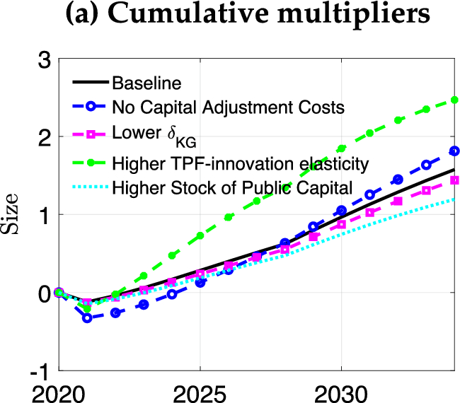
Additional simulations. This figure shows the NGEU multipliers, with , in our baseline simulation and under alternative calibrations
Crowding-out effects of the fiscal stimulus. One of the reasons why a fiscal stimulus may have limited effects might be that it has crowding out effects. Namely, the increase in prices generated by the fiscal stimulus may lead to a reduction of privately funded investment into physical capital or innovation. To illustrate this, we make use of the counterfactuals where all the funds are allocated either to innovation transfers or to capital transfers, as described in Sect. 4.3.
Starting with the case where all funds are allocated to innovation expenditures, the left panel in Fig. 6 shows the path of transfers as a share of initial BGP innovation expenditures and the dynamics of total innovation expenditures. In this scenario, transfers amount to roughly per year of what is spent on innovation in the initial BGP. Note, however, that total innovation expenditures increase by less, peaking at around . This means that there is indeed a substantial crowding-out, even though not complete, which limits the expansionary effects of the fiscal stimulus.
A similar story holds when we look at the scenario where all funds are allocated to capital transfers, plotted in the right panel. Here, we plot transfers as a share of the initial BGP level of investment and the dynamics of total private investment in physical capital. Since the BGP investment in physical capital is much larger than innovation expenditures, now transfers represent a smaller share when plotted against BGP investment. Yet, we still observe a similar crowding out effect, with transfers representing but total investment peaking at around , which partly explains the small effects of capital transfers on GDP reported in the main text.
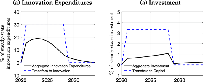
Crowding out of fiscal stimulus. Left panel: considers the simulation where all NGEU funds are allocated to innovation transfers. It shows transfers and total innovation expenditures as a share of initial steady-state innovation expenditures. Right panel: considers the simulation where all NGEU funds are allocated to capital transfers. It shows transfers and total investment in physical capital as a share of initial steady-state private capital
Alternative spending paths. Our baseline spending path for NGEU spending considers a uniform disbursement of funds, as described in Sect. 4.1. In this section, we evaluate the consequences for output of alternative paths for the disbursement of funds, which could be of interest given potential delays in the implementation of the NGEU program.
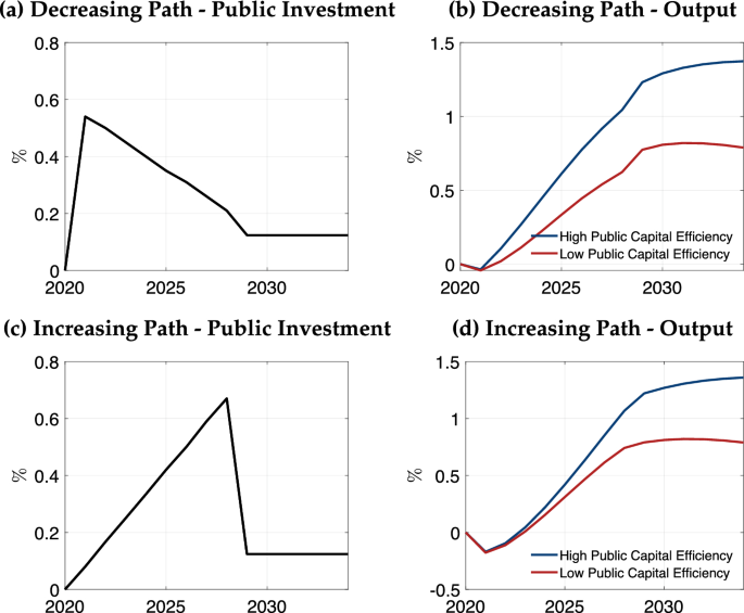
Alternative spending paths. This figure shows the output effects under alternative paths for public investment. The top row considers a decreasing path for public investment (panel a) and the corresponding effects on output (panel b). The bottom row considers a decreasing path for public investment (panel c), and panel d shows the corresponding path for output
We consider two alternative paths for public investment, the largest component of the NGEU funds according to our baseline. Namely, we entertain a decreasing path for public investment, as depicted in panel (a) of Fig. 7, and an increasing path for public investment, shown in panel (c).
In the medium run, the total effects on aggregate output of the different spending paths are quite similar, compare panels (b) and (d) of Fig. 7. This should not come as a surprise given that in all scenarios we maintain fixed the overall size of the program, as well as the allocation of funds to the different fiscal instruments. Indeed, the average effect on GDP growth (not shown here) remains the same under these alternative paths as under our baseline flat spending profile. The timing of the stimulus differs across the different spending paths, however. A decreasing path for public investment (bottom row, Fig. 7) implies an output effect that is more front-loaded than in our baseline, while the stimulus to output under the increasing profile (top row, Fig. 7) is more back-loaded.
Rights and permissions
Reprints and permissions
About this article
Cite this article
Domínguez-Díaz, R., Hurtado, S. & Menéndez, C. Fiscal stimulus and productivity: simulating the NGEU program with an endogenous growth model. SERIEs (2025). https://doi.org/10.1007/s13209-025-00304-1
- Received
- Accepted
- Published
- DOI https://doi.org/10.1007/s13209-025-00304-1
Keywords
- Productivity
- Public investment
- Endogenous growth
- Next generation EU
JEL Classification
- O38
- O52
- O40
- H54
- E65