The current global climate emergency has highlighted the urgent need for sustainable practices across all industries, including logistics. As recognised by the Conference Of the Parties (COP 21) (Klein et al. 2017), climate change represents an urgent and potentially irreversible threat to human societies and the planet. It is crucial to accelerate the reduction of global greenhouse gas emissions and also pollutant emissions. The movement towards cooperative multimodal logistics has become increasingly important as companies aim to reduce their environmental impact while maintaining efficient supply chains. The approach presented in this document emphasises collaboration and shared resources among different transportation modes, such as road, rail, maritime and air transport, to achieve a more sustainable and resilient logistics network. In fact, to address environmental challenges, it is crucial to consider managerial implications and perspectives on how the proposed methodology aligns with the current global climate emergency. Furthermore, we focus on how utilising vehicles that are not operating at full capacity thus contributes to reducing the overall number of vehicles on the road according to a green-oriented vision. This strategy aligns with the overarching goal of minimising the environmental impact of logistics. Subsequent sections will delve into experimental results, suggesting that even minor adjustments to the multimodal network can lead to significant reductions in pollutant emissions. These findings outline the potential environmental benefits of optimising existing transportation resources. Finally, the importance of sharing information, preserving confidentiality, integrity (Kale 2024; Ogiela 2010, 2013) and resources throughout the supply chain has become crucial for ensuring efficient and sustainable operations. Over the past 20 years, there has been increasing recognition of the environmental and social impacts of logistics, in addition to traditional economic considerations. As a result, the termsgreen “logistics” and “sustainable logistics” have emerged as pivotal concepts in both industry and academic research (Fareed et al. 2024; Jazairy 2020). Previous research has indicated that the integration of Industry 4.0 technologies (ITE) and the adoption of green practices may serve as catalysts for progress toward a sustainable economy (Sharma et al. 2023; Zaare Tajabadi and Daneshvar 2023). These terms encompass a range of practices aimed at reducing the negative environmental and social impacts of logistics, including reducing emissions, minimising waste, and promoting ethical labour practices (Zhao et al. 2020). The investment in managing economic, social, and  emissions helps protect the environment, reduce total transport costs, and ensure sustainability (Alsarhan et al. 2021), which is the main objective of this article.

In recent times, there has been a heightened acknowledgement among professionals and specialists regarding the imperative to prioritise multimodal transportation, driven by its diverse sustainable advantages (Labarthe et al. 2024; Jiang et al. 2020). This emphasis aligns with the overarching goal of mitigating congestion, air pollution, and consequently, noise and infrastructure deterioration (Ambrosino and Sciomachen 2021). Moreover, there is growing attention to studying and researching the organisation of different cargo types within the realm of multimodal transportation. It should be noted that the multimodal delivery of specialised cargo carries significant responsibility, especially considering the distinct properties inherent to such cargo categories. Given that multimodal delivery involves the use of at least two modes of transport, it requires adherence to specific regulations governing cargo transportation for optimal efficiency and safety (Orozonova 2022). The European Union (EU) has also recognised the negative externalities associated with road haulage, such as delays, congestion, and the environmental impact of  emissions (Ambrosino et al. 2019; Molloy et al. 2021). To address these issues, the EU has set ambitious targets for a competitive and resource-efficient transport system, including a shift towards more sustainable modes of transport like rail and waterway transport (Bharti 2025; Alkaissi et al. 2024). This modal shift represents a crucial step towards reducing the environmental impact of the transport sector while ensuring efficient and reliable transport of goods (Gohari et al. 2022; Nassar et al. 2023). By diversifying transportation modes and promoting sustainable practices, the transportation sector can make a significant contribution to the broader goal of achieving a more sustainable and resilient economy (Cerrone and Sciomachen 2022). Vosough et al. (2022) address the significant issue of road traffic, a major contributor to air pollution that poses a serious challenge in numerous large cities. To address this concern, they employ a dynamic traffic network simulator. This simulator models decisions related to the mode of transportation, departure time, and route choices. Comi and Polimeni (2020) conducted a study aimed at examining the viability of short-sea shipping (SSS) services as an eco-friendly freight transportation system that can meet economic, social and environmental requirements. They developed an evaluation system to assess the capabilities of SSS and the general advantages associated with reduced external costs. The findings of their research support the notion of transitioning freight transportation away from less environmentally friendly road transportation and toward more sustainable SSS methods to achieve greater external benefits. Okyere et al. (2022) evaluated a sustainable multimodal freight delivery system that integrates road, rail, and waterway transportation in Ghana. They used a genetic algorithm model to formulate an optimal system that mitigates economic, social, and environmental issues. The Sustainable Multimodal Freight Transport and Logistics System (SMFTLS) model can assist policymakers in making informed decisions about the appropriate transport schemes for freight transportation. Developing rail and waterway infrastructures can help establish a resilient and sustainable system to manage the growing demand for freight transportation. Zheng et al. (2022) focused on the integration of cold chain logistics (CCL) with multimodal transport in China, combining land and sea transportation into a unified transport chain. The study aims to efficiently select the best logistics route to deliver cold chain foods (CCFs) by analysing and integrating the characteristics of multimodal logistics and CCL. To utilise the model, an improved particle swarm optimisation (IPSO) algorithm is introduced, which has proven to be both fast and accurate in solving the problem. Sensitivity analysis is conducted to assess the impact of variations in railway speed and cost on path selection. The results indicate that railway transport is preferable to highway transport for medium and long distances. Ambrosino et al. (2018) highlight the importance of intermediate facility locations in multimodal freight distribution networks and their impact on external costs. The study uses real data from a port system network serving inbound container flows in Italy and evaluates the impact of sustainability external costs on the design and management of the network. In the study conducted by Dong et al. (2020), it is demonstrated that multimodal distribution is not only environmentally friendly but also economically advantageous, particularly when multiple industrial stakeholders collaborate to establish economies of scale. The article emphasises how this approach could contribute to mitigating the air pollution and road congestion associated with automobiles in India. The authors illustrate how the mixed-integer programming (MIP) model can be employed to provide decision support through a case study on automobile distribution, leveraging the extensive coastline for maritime transportation opportunities. Specifically, the study addresses the escalating environmental emissions linked to automobile transport, resulting from rapid economic development, and proposes a modal shift solution involving the replacement of a portion of road transport with roll-on roll-off (RoRo) ships. A similar study is undertaken by Garrido et al. (2023), who provide an appropriate framework for assessing several hypothetical transportation scenarios. They address the logistic performance challenges of using Bogotá as the main hub for shipping goods to other destinations in Colombia. The determinant factors encompass excessive truck traffic, low density of railways in service, and no accessible river routes. The article proposes a balanced linear transshipment (BLT) model to estimate the optimal multimodal freight transportation network from the mentioned city to seven main destinations in the country. Recent studies also highlight the increasing awareness of the positive impact derived from the adoption of an electric fleet in last-mile logistics operations (Rafael et al. 2023). In the work by Alarcón et al. (2023), the authors outline the importance of electric vehicles (EVs) as a pivotal solution to the climate change problem. Their objective is to identify the main themes and prospects associated with electromobility and freight logistics, with the objective of identifying potential directions for future research in the field of sustainable development. The article by Han (2023) focuses on the role of robots in the logistics sector. This research addresses the challenge of path planning and control for logistics robots in complex environments. The proposed method begins with the use of a convolutional neural network (CNN) to learn feature representations of objects within the environment, enabling object recognition. Subsequently, the Dijkstra algorithm is employed for path planning, ensuring the selection of optimal shortest paths across diverse scenarios. The shortest path problem is one of the most studied optimisation problems in the literature, and it is of crucial importance, especially for logistics-related problems. Unlike the classic shortest path problem, the variant we will address includes temporal constraints to facilitate the cooperation of multiple vehicles. Additionally, the use of the edges associated with a vehicle requires an activation cost. Within the family of Constrained Shortest Path Problems (Festa 2015), the Time-Constrained Shortest Path (Liu and Huang 2022) is a crucial reference for our work. Additionally, activating a vehicle can be considered as employing a specific colour for the k-Colour Shortest Path Problem (Cerrone and Russo 2023). To the best of the authors’ knowledge, there is no existing variant of the shortest path problem that combines temporal constraints with activation costs for edge sets. For this reason, this paper introduces a mathematical model capable of modelling this variant of the shortest path problem. In this paper, a multimodal logistics problem is defined in which we have to intersect the paths of different carriers to transport units of goods from a given origin to a destination. The optimisation of the route, when a customer must ship its goods, is based on a set of multimodal routes offered by a set of carriers. More precisely, the optimal choice considers several parameters orientated towards the paradigm of cooperative logistics and the green impact. The applied scenario involves a framework able to gather information on a series of transports carried out by vehicles of different types (trucks, trains, ships, etc.). These scheduled journeys from an origin to a destination pass through several stages. For each of these transports, this framework collects information on travel times, the type of transport mode and related vehicle, and the payload capacity that is not yet occupied and can be made available for other transports.

The purpose of this study is threefold:

1. a.Verify whether the available payload capacity of already scheduled journeys can be used to satisfy a new request to transport goods from an origin to a destination without requiring additional vehicles;
2. b.See how many transshipments from one vehicle to another are necessary to reach the destination;
3. c.

   Compute the transport cost, in terms of both direct and indirect costs, related to the environmental impact of the defined routes.

Thus, the overall objective of sustainable logistics is pursued in this research work not only by minimising the number of vehicles on the road, and thus the traffic, in multimodal transport networks, but also by trying to offer shippers the least polluting mode of transport to travel the routes required for their deliveries. Note that we used the Handbook on the External Cost of Transport (Delft et al. 2020) to determine the impact of environmental pollution. In the proposed approach, we assume that we know the list of routes offered by various transportation companies and their operative vehicles for each transport mode. We then compute the minimum-cost origin–destination paths in a multimodal logistic network model specifically designed for the present problem. The remainder of this work is organised as follows. Section 2 details the problem while providing an example of the set of available transportation routes to derive the multimodal path. The definition of the underlying multimodal graph G is also given. Section 3 introduces the mathematical programming model to identify the optimal solution to the problem. Section 4 reports the experimental results of the tests conducted to validate the proposed approach and highlight the unique characteristics of the problem. Finally, some conclusions and outlines are given for future work.

The application scenario for this study involves multiple carriers that conduct their shipments without necessarily fully utilising their cargo capacity; therefore, they have the opportunity to share part of the available cargo space and optimise their journeys. Carriers make available information on scheduled routes and the available cargo space for each route to optimise load and increase profits. Specifically, when sending goods from one origin to a destination, the aim is to exploit the possibility of not using a dedicated vehicle but rather using the available cargo space on the routes offered by already active carriers. In this way, three different objectives can be achieved: (i) to reduce transportation costs; (ii) to decrease the amount of pollution produced; and (iii) to allow the fleet to optimise its assets.

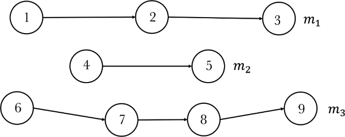
An example of a graph R with three different routes, namely , , and , respectively, traveled by vehicles , , and 

Full size image

Let R be the set of routes that the carriers must take. Then  (, ) is a digraph consisting of a set  of nodes, representing the physical locations visited on the routes, and a set  of arcs, representing the available connections between nodes. Each arc  is associated with the vehicle  travelling the corresponding route, in such a way that  denotes that the path from node i to node j is travelled by vehicle k. Let M hence denote the set of vehicles involved in the delivery schedule. From Fig. 1, we can see that the paths offered by different carriers always have an initial node (nodes 1, 4, and 6, respectively, in Fig. 1), a final node (nodes 3, 5, and 9, respectively, in Fig. 1), and possibly several intermediate nodes that represent the stops made by the carriers before reaching their destination (nodes 2, 7, and 8, respectively, in Figure 1). A weight  representing the related travel time is associated with the arc . Moreover, for each arc it is necessary to define the emissions cost produced by vehicle k (), the fuel transportation cost (), the service cost () (including loading the cargo and maintenance), and the consolidation cost () between the nodes i and j. As a novel issue of the representation of the multimodal logistics network, an additional set of arcs, denoted D, representing all possible detours between nodes, is considered. An example of a multimodal network with detours is shown in Fig. 2.

Definition 1

A detour is a deviation from the original route that a vehicle is willing to take to pick up goods from or deliver goods to a location different from its original destination.

Note that each carrier can specify the level of allowed detour for each route. For example, a truck may be willing to deviate a few kilometres from its route to pick up an item. The maximum number of kilometres within a detour offered for each route is an integral part of the input of the problem and is defined by the carriers providing the routes. The cost per kilometre of the detour is also part of the problem input.

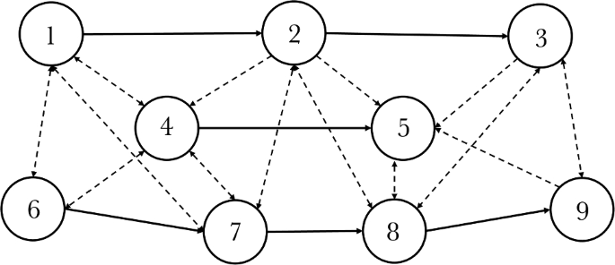
Example of a multimodal graph, where dashed edges represent potential detours that allow the goods to be moved from one vehicle to another

Full size image

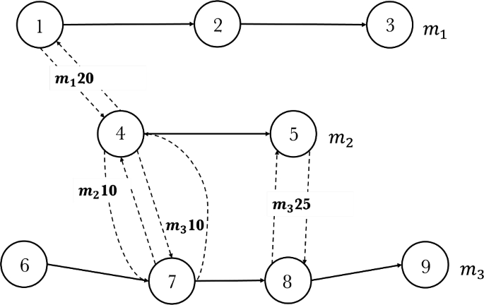
Example of a multimodal graph, where dashed edges represent admissible detours

Full size image

Figure 3 shows an example of a multimodal network that has only admissible detours. In the given example, we assume that vehicle  allows up to 40 km of detours, vehicle  allows up to 20 km of detours, and  allows up to 50 km of detours. It is worth noting that there are four edges between nodes 4 and 7, meaning that both  and  can offer detours between these nodes. Note that not all means of transport allow detours. Admissible detours are formally defined as follows.

Definition 2

Admissible detours are those routes travelled by carriers who have declared their availability for the detour and whose length does not exceed the maximum length allowed.

Figure 4 shows the same three routes with admissible detours depicted in Fig. 3, with the addition of nodes o and d, representing, respectively, the origin and destination nodes associated with the customer’s request for transport in graph R. In fact, when calculating a multimodal path for a specific request, nodes o and d must be added to the set of routes offered by the carriers. Moreover, two additional subsets of arcs must be added to R. More precisely, let  be the set of outgoing arcs from node o, indicating that the customer is willing to travel the corresponding distances to deliver the goods to a carrier node. Analogously, let  be the set of arcs entering the destination node d.

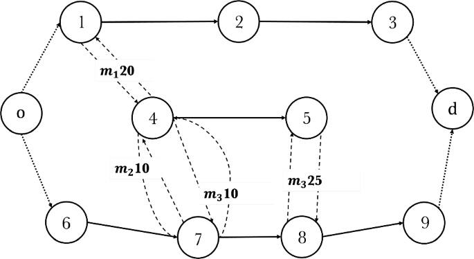
Example of a multimodal graph to which origin and destination nodes associated with the customer’s transport request have been added

Full size image

To model the present problem, we then use the digraph , where  is the set of nodes that contains all the stops associated with the routes offered by the carriers, the origin of the goods to be shipped and their destination.  represents all the arcs of the graph and, therefore, all possible movements of the goods using the vehicles in the set M.

To represent the main features of multimodal route problems, we must deal with models capable of including all the parameters that can affect the corresponding decision process. Thus, the digraph  defined above with the following specifications is considered as the underlying network model:

• V: set of nodes.
• E: set of oriented arcs.
• M: set of vehicles.
• : origin node.
• : destination node.
• q: quantity to be transported.
• : available capacity for each vehicle .
• TC: truck capacity.
• ta: maximum time to arrival at node d.
• : travel time for vehicle k to move from node i to j.
• :  emissions cost of vehicle k from node i to j.
• : service cost of vehicle k.
• : fuel transportation cost of vehicle k from node i to j.
• : cost of load consolidation of vehicle k from node i to j.
• : departure time of vehicle k from node i, .

Furthermore, we use the multiplier  associated with the cost  to weigh the role that the emissions cost plays in the overall cost differently. In fact, throughout the article, we will explore how the variation of  influences the performance of our approach and analyse the practical implications of this choice in the proposed system design. This problem has been modelled using mixed-integer linear programming (MILP). As a result, the proposed solution will require, in the worst case scenario, an exponential amount of time dependent on the input size, the MILP being classified as an NP-complete problem (Kannan and Monma 1978). Our MILP model has the following decision variables:

As already mentioned, the objective function (of) of the problem aims to minimise the following four cost components:

1. a.Costs associated with  emissions. These costs refer to expenses incurred due to the emission of  during transportation.
2. b.Service cost of the used vehicle. This cost represents the expenses associated with the use of a specific vehicle for transportation.
3. c.Transportation cost. This cost includes fuel costs.
4. d.Consolidation cost. This cost is considered only for the road mode of transportation. It refers to the expenses incurred to consolidate goods into a single truckload for more efficient transportation.

Consolidation of the load in transportation involves optimising the available space to transport the maximum amount of goods while avoiding under-utilisation of capacity. To encourage our mathematical model to generate solutions that prioritise load consolidation, we have introduced the concept of consolidation cost as a penalty to be applied when the load is not well consolidated. We have defined the function (1) to calculate this cost. The cost is associated with each arc used in the solution and can have a maximum value equal to one-tenth of the transportation cost. Specifically, we calculate the percentage of unused load capacity, which ranges from zero (when the cargo capacity is filled to 100% capacity) to one (when a truck travels with an empty load). To consider this percentage, we use the parameter TC, which represents the capacity of the trucks. The parameter is calculated based on the trucks’ capacity because load consolidation applies only to trucks:

Then, the present problem can be formulated as follows:

subject to the constraints

The objective function (2) consists of the four previously defined cost components. Equation (3) ensures that if a vehicle reaches a node j that is not the origin or destination, it must also leave that same node. Constraint (4) ensures that from the origin node o, the vehicle must exit to transport the goods. Constraint (5) ensures that the vehicle must reach the destination node d. Constraint (6) allows the use of the arc (i, j) with vehicle k only if vehicle k is active in the solution. Constraint (7) is formulated so that if the variable  is equal to zero, the left-hand side of the inequality takes a value greater than the arrival time at the destination, thus always satisfying the constraint. However, when the arc (i, j) is traversed by vehicle k and the corresponding  is active, in order to satisfy the constraint, the departure time from node j must be greater than the departure time from node i plus the corresponding travel time. Finally, in (8) and (9), the decision variables are defined.

3.1 Proposed approach

This subsection presents the procedure (Algorithm 1) used to solve a single instance of the problem. Step 2 of the procedure is necessary to create the set of routes  by removing from R all routes with residual cargo spaces less than q. The next step uses the procedure CreateGraph(R, o, d, RaDis) to construct the graph G used by the mathematical model. This procedure is detailed in Section 2. The mathematical model of step 4 computes the optimal solution to the problem represented by graph G.

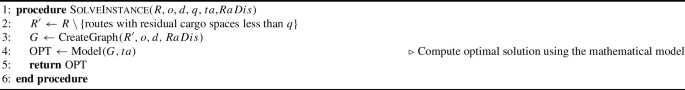
Procedure to Solve a Single Instance of the Problem

Full size image

The following is a description of what it does:

1. 1.The algorithm takes several Input parameters:
   • R: Set of routes.
   • o: Origin.
   • d: Destination.
   • q: Quantity to be transported.
   • : Time of arrival.
   • RaDis: The maximum distance the customer who needs to ship their goods is willing to travel.
2. 2.Remove routes from R where the residual cargo space is less than q, denoted as .
3. 3.Create a graph G using the modified set of routes , origin o, destination d, and RaDis.
4. 4.Use a mathematical model to calculate the optimal solution (OPT) based on the graph G and the arrival time ta.
5. 5.Output: Return the optimal solution OPT.

This section presents the experimental results of the tests conducted. First, we will illustrate how the test instances were generated and how the associated costs were defined. Then, we report the experimental results and provide an analysis. It is important to note that the code was implemented in Java and the mathematical models were solved using the CPLEX solver, version 20.1.0. The underlying idea of the tests conducted is not to analyse the performance of the utilised mathematical model but to examine the problem to determine whether a multimodal approach, where the available load capacity of the travelling vehicles can be used, is advantageous in a real-world context. To achieve this, we generated realistic scenarios and performed experimental tests varying the main generation parameters. We did not conduct tests related to the computational performance of the model, as our problem is based on identifying a single multimodal route, and for this problem, the integer linear programming model did not require more than ten seconds to produce the optimal solution for any of the 648 instances.

4.1 Instances

This subsection explains how the 648 test instances used in this work were generated. The experiments were conducted by varying the parameter  and by including or excluding the consolidation cost, necessitating a total of 3,240 computational tests. First, we created 18 different multimodal example graphs (see Fig. 3). The generation of these graphs involved the systematic variation of three key parameters: the total number of routes offered by the carriers, the percentage distribution of different vehicle types (truck, train, plane, ship), and three different random seeds. All details of the test instances are shown in Table 1, where the column headings are as follows: Vehicles consists of four values associated with the percentage of truck (Trk), train (Trn), aeroplane (Pln), and sea (Shp) routes offered by the carriers; R is the total number of offered routes; and # Routes is the number of generated routes per vehicle type.

The route generation was implemented realistically across all provinces in the Italian territory. For each of the 107 Italian provinces, we used the city centre as the starting point of the routes. The R routes are generated between random pairs of provinces by randomly selecting (with the probability distribution outlined in the Vehicles parameter) the type of vehicle. A search was conducted for each Italian province to identify whether there was a railway station, airport, and seaport, to determine the type of vehicle compatible for each province. This ensures that the creation of an arc between two nodes for a specific vehicle type only occurs if both nodes (associated with the provinces) accept the same types of vehicles. The resulting routes are reported in Fig. 5a. Additionally, the algorithm was implemented to prevent land vehicles from connecting provinces located on the islands of Sardinia and Sicily. As can be observed in Fig. 5a, only sea routes (solid grey lines) and air routes (dotted grey lines) connect the islands with the rest of the Italian peninsula. In these graphs, only trucks are allowed to take detours, and the detour distance for each truck varies randomly within the range of 20–80 km. For each of the 18 multimodal scenarios in Table 1, we generated 36 instances for a total of 648 test cases. Each instance varies in terms of the number of items shipped (Items), the origin–destination (see Fig. 5b), and the shipping radius, as reported in Table 2. The shipping radius (RaDis) refers to the maximum distance that the customer who needs to ship their goods is willing to travel. The tests were carried out considering three different requests with the following origin and destination cities: Reggio Calabria to Terni (RC-TR), Roma to Bolzano (RM-BZ), and Taranto to Torino (TA-TO). We selected these three requests to cover different Italian regions and evaluate the performance of the model in various geographical contexts. Additionally, each route presents unique infrastructure characteristics, such as the prominence of rail or highway networks, allowing us to test the model’s adaptability across diverse logistical infrastructures within Italy. Table 2 shows that, as the generation parameters (Items, RaDis) vary, not all instances are feasible, since it is not always possible to connect the origin and destination using multimodal paths because the vehicles do not have enough available space to carry the required goods (Items) or because there is no multimodal path that reaches the destination. In particular, it becomes evident that as the number of items dispatched increases, the number of multimodal routes that can be used decreases due to the limited residual space available in some transportation modes. Consequently, the number of infeasible solutions increases. On the contrary, as RaDis increases, it becomes feasible to use more routes, even those that are not in close proximity to the demand origin. Therefore, with increasing RaDis, the number of feasible solutions increases correspondingly.

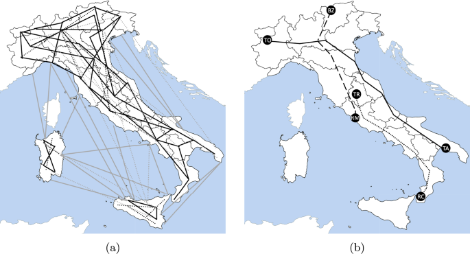
Visual comparison of the set of routes offered by carriers 5a and specific routes representation 5b

Full size image

The costs used in our experiments were derived from a small market survey conducted among a series of small transport operators operating in Italy. The costs were estimated by the operators, who specified that as the number of requests increases, the costs may undergo significant changes. For each mode of transport, a cost per km (transport cost) and a cost per use (service cost) of the vehicle were included. The service cost is associated with the loading-unloading operations of the goods and possible cargo reorganisation. Table 3 shows these costs. The costs, of course, depend on the type of vehicle used for transportation, the load transported, and the technology used. It is important to note that these are only average values and that the following costs can vary significantly depending on the specifications of each vehicle and the conditions of use. The conversion of  costs into euros depends on the carbon emission value set in the European Union Emissions Trading System, as reported in (European Energy Exchange 2023). On the other hand, the consolidation cost was calculated using the formula (1), with the truck capacity fixed at .

Throughout the study, the pallet was chosen as the load unit. For this load unit, it was decided to calculate the consolidation cost only for trucks, as shipments of a few pallets would not significantly impact ships, aeroplanes, or trains considering their high carrying capacity. However, for trucks, the goal is to maximise their load capacity. Formula (1) calculates the ratio between the remaining space in the truck after loading the goods and the total capacity of the truck. This ratio is then multiplied by one-tenth of the transportation cost.

4.2 Results

In this subsection, we present the results of the analysis of the proposed multimodal transportation framework. Our analysis focused on evaluating the performance of the system in terms of cost, environmental impact, and efficiency. The results provide insights into the effectiveness of different combinations of modes in meeting transportation needs, helping to identify the most promising options to reduce costs, minimise carbon emissions, and improve overall performance.

Table 4 presents the average costs associated with the objective function for each of the different scenarios analysed presented in Table 1. In these scenarios, we have varied both the number of items to be shipped and the maximum delivery radius that the customer is willing to cover to have their goods delivered by the available carrier. An immediate observation is that when the customer’s delivery radius (RaDis) is set to 0, the costs are higher. This occurs because in this case, the optimal route can only start by utilising those carriers that pass directly through the origin of the shipment or allow a detour to pick up the items. Naturally, the detour offered by the carrier impacts the objective function. Conversely, when we set RaDis at 100 km, we notice a significant decrease in costs, in all the routes considered and for all numbers of shipped items. This happens because we have observed that as the delivery radius increases, the customer can access multiple carriers and can choose the most cost-effective option. Note in particular that in the case of an item transported from Reggio Calabria to Terni, by increasing RaDis to 100 km, we achieved savings exceeding 57%. It is important to emphasise that costs increase proportionally to the number of items to be shipped. These results highlight the significant impact of RaDis on the total shipping cost. Since the parameter RaDis is directly chosen by the customer requesting transportation, informing them about the impact of this parameter is crucial in implementing a multimodal logistics system. Of course, the number of items to be shipped also has a significant impact on costs, but this parameter is an unmodifiable input of the problem. The details of the individual cost components of the objective function are presented in Tables 5, 6, and 7, respectively, for the Reggio Calabria-Terni, Roma-Bolzano, and Taranto-Torino routes. Analysis of the results in Table 5 reveals notable cost variations in different scenarios for the Reggio Calabria-Terni route. The table presents the individual components of the objective function, namely Emissions, Service, Transportation, and Consolidation. All values are averages for the 18 test scenarios. These variations highlight the importance of considering factors such as the number of items shipped and the maximum distance customers are willing to travel. In general, as the number of items shipped increases, there is a gradual decrease in the emissions costs (Emi). This can be attributed to the potential consolidation of goods, resulting in more efficient and environmentally friendly transportation.

The service cost (Serv) shown in Table 6 indicates that a moderate increase in the parameter RaDis does not lead to a reduction in this cost. However, a significant increase in RaDis up to 100 km results in a substantial reduction of service costs by approximately 20%. On the other hand, the consolidation cost (Con) shown in Table 5 and Table 6, decreases progressively as the parameter RaDis increases. For example, in Table 6, when sending a single item with RaDis equal to 10, 50, and 100, compared to RaDis equal to 0, we observe reductions in the consolidation cost (Con) of 34%, 57%, and 80%. The behaviour of the consolidation cost with increasing RaDis shows a slightly different pattern in Table 7. The decrease in the consolidation cost as RaDis increases is confirmed for values of RaDis greater than 10 km. However, there is a moderate cost increase when transitioning from RaDis of 0 to RaDis of 10 km. This is mainly due to the presence of the port and the Taranto train station. With , the use of ships or trains for initial movement is highly favoured, resulting in a decrease in the consolidation cost since these types of vehicles do not incur consolidation costs. Table 8 shows the average kilometres travelled for each vehicle type, grouping the instances based on the average types of vehicles present in the scenario.

Considering the uniform distribution (25-25-25-25) of vehicle types, with an equal number of routes for each vehicle type, we can immediately observe that road vehicles are the most used means of transportation. This holds true in other scenarios as well. In the 50-20-15-15 scenario, where there is a 100% increase in the number of routes offered by trucks, there is only a 14% increase in the kilometres travelled by road vehicles. Similarly, in the 70-10-10-10 scenario, where there is a 180% increase in the number of routes offered by trucks, there is only a 10% increase in the kilometres travelled by trucks. As a direct consequence of the increased routes offered by trucks, there is a decrease in the kilometres travelled using other modes of transportation. An expanded selection of truck routes facilitates the identification of direct paths, resulting in reduced overall mileage and a reduced requirement for additional vehicles.

Tables 9, 10, and 11 present the average cost value associated with the solution and its components, grouping the 648 instances differently for each table. Specifically, Table 9 groups the instances according to the distribution of vehicle types. In Table 10, the instances are grouped according to the number of items transported, while Table 11 groups the data according to the values of RaDis. Analysing Table 9, it is interesting to note that as the percentage of truck-operated routes increases from 25% to 50%, the objective function and the value of the emissions cost increase slightly. However, when the rate of truck-operated routes in the instances is increased to 70%, both the solution cost and the emission cost decrease significantly. Table 10 is particularly interesting, as it helps us understand the impact of the number of items transported on the final cost of solutions. Naturally, the cost increases as the number of items transported increases, but at the same time, the emissions remain constant or slightly increase. Table 11 confirms that as the value of RaDis increases, the average cost of the solutions decreases drastically. This clearly implies that if the customer who needs to send their items is willing to travel, he can choose from better and more competitive transport offers.

Table 12 presents the average kilometres travelled per instance for different modes of transportation, varying the parameter RaDis. This table is crucial, mainly when analysed together with Table 11. As RaDis increases, the cost of the solution decreases significantly, but at the same time, the kilometres travelled do not decrease significantly. This is because, with a wider search radius to select the initial mode of transportation, the choice is often made to use ships, trains, or planes. The increase in the kilometres travelled by ship or train justifies the cost reduction, especially in terms of associated emissions. The graph in Figure 6a shows that as RaDis increases, more cost-effective modes of transportation compared to truck transport can be chosen. It is also interesting to note that when  km, trains and ships are preferred over planes.

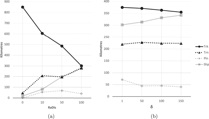
For each type of transportation, a line shows the average kilometres travelled as the considered parameter increases: 6a based on RaDis, and 6b based on the emission cost

Full size image

Table 13 shows the results in which the multiplier  associated with the emission costs was varied to assess its impact on the choice of transportation modes. As defined in Section 3, we introduce the term  as a multiplier associated with the cost . As stated previously,  is used to weigh differently the role played by emissions costs in the overall analysis. In practice, the parameter  allows us to modulate the relative importance of emission costs in relation to all components of the objective function. Note that a higher  value will place greater emphasis on the impact of emissions costs, while a lower value will reduce their influence. Thus, this weighting mechanism provides flexibility in configuring the model, allowing for more precise customisation based on the specific needs of the application or context. The values of  considered were 1, 50, 100, and 150. Considering that the emissions costs used in this study were derived from (Delft et al. 2020), the use of the parameter  to increase the impact of emission costs is extremely useful for investigating the existence of more sustainable solutions to the problem. The results, reported in Table 13, thus demonstrate that as  increases, the model tends to reduce the usage of trucks and planes, favouring instead trains and ships. Specifically, the average kilometres travelled by trucks (Trk) decrease as  increases. The graph in Figure 6b shows that the average kilometres travelled by trains (Trn) remain relatively stable or increase slightly. In addition, the use of the plane model (Pln) significantly decreases, while the ship model (Ship) experiences a substantial increase. These findings indicate that the increase in emissions costs has influenced the choice of transportation modes, with a greater inclination toward more sustainable options such as trains and ships. This underscores the importance of considering emissions costs in optimising transportation routes to minimise the overall environmental impact.

To investigate the impact of the consolidation cost on the solution, we performed tests on the 648 instances, fixing the consolidation cost to zero. Table 14 shows the results obtained by comparing the scenarios with and without the consolidation cost. Our focus was on two specific parameters: Load90, which indicates the number of transports carried out using trucks that were filled to at least 90% of their capacity, and Fullness, which represents the average occupancy of trucks. Table 14 shows the computational results obtained while varying the parameters (Vehicles, RaDis, Items). In particular, three scenarios for Vehicles, four scenarios related to RaDis, and three scenarios associated with the number of items transported are considered. As shown, the number of trips with trucks that were at least 90% full increases from seven, without the consolidation cost, to 20 when consolidation costs are considered, thus tripling this kind of route. For the same cases, with respect to the fill percentage, it increases from 58% to 63%, resulting in a 5% increase in load occupancy. Furthermore, it is interesting to note that the fullness increases from 59% to 67% when the parameter RaDis is increased, indicating that when the customer is willing to travel longer distances to choose the optimal starting points, the consolidation of transports can be significantly improved.

This paper presented research based on the determination of minimum cost origin–destination routes on ad-hoc-defined multimodal graphs. The proposed MILP model and related data management procedures have been integrated into a single framework that aims to select the route that minimises the total cost of transportation by optimising logistics operations within a multimodal transportation network. In fact, the proposed work addresses the need to carry out logistics practices in a sustainable manner due to the global climate emergency.

The proposed framework determines the optimal route by considering factors such as vehicle load utilisation, transshipment capability, and transportation costs, taking into account not only the monetary cost, which depends on the length of the route and the vehicle used but also the cost of pollutant emissions and the level of vehicle occupancy. One innovative aspect, in fact, consists precisely of the introduction in the objective function of the so-called consolidation cost model, which tends, as the results have shown, to minimise the total kilometres travelled by road vehicles, favouring trips made by fully loaded trucks. The framework incorporates parameters aligned with the principles of cooperative logistics and environmental impact for different types of vehicles, such as trucks, trains, planes, and ships.

Through extensive tests performed with about 3,240 instances, we have demonstrated the effectiveness of the proposed MILP model, based on an ad-hoc-defined multimodal graph, in accounting for the aspects mentioned above. We can observe, for example, that in scenarios in which the customer’s delivery radius was set to within 100 km, the average cost of the solutions is significantly lower than it is for longer-haul routes, even though the total distance travelled remains almost unchanged. This is because, in the search for the optimal solution, customers are given access to more competitive transportation options. An analysis of these results underscores the importance of cooperation among multiple carriers within the multimodal network. Specifically, by allowing various carriers to share unused cargo space in already scheduled routes, the proposed framework reduces the need for additional vehicles and leverages existing capacity to accommodate new demands. This cooperative approach decreases the total number of vehicles required, reducing both transportation costs and emissions, thus aligning with the sustainability goals of the framework. An even more significant result from an environmental sustainability policy perspective emerged from the tests performed by varying the weight given in the objective function to the cost component based on pollutant emissions. In fact, it emerges that as the weight given to this cost increases, the use of trucks and planes decreases, favouring the use of trains and ships. Specifically, the average kilometres travelled by trucks decrease as the emissions cost coefficient increases. Another result to highlight relates to the tests performed to investigate the impact of the consolidation cost on optimal solutions. In fact, it was observed that by considering a penalty for road trips made by trucks that were not fully loaded, the percentage of trucks that were nearly 90% loaded can be almost tripled. Furthermore, an average increase of at least 8% is found when there is a willingness to take slightly longer routes to consolidate loads.

Therefore, by analysing the results obtained by the proposed MILP model, we can say that our framework is definitely a valuable starting point to be pursued in order to promote incentive policies and strategies for sustainable logistics, providing valuable insights for decision-making in scenarios of real demands for medium- to long-haul transportation of goods. In summary, cooperation proves crucial in making logistics networks more resilient, reducing emissions, and achieving cost efficiency, making it an essential focus for sustainable logistics practices.

5.1 Future scope

Within the ongoing collaboration with the Joint Research Centre (JRC) of the European Commission, the future scope of this research will involve a thorough evaluation of the proposed model using datasets and instances provided by the JRC. The primary objective is to rigourously reflect TRIMODE (TRansport Integrated MODel of Europe) data. TRIMODE is a comprehensive modelling system designed to encompass various scenarios related to infrastructure investment, pricing, technology, and regulatory policies. The model seamlessly integrates a detailed European transport network model with advanced energy and economic models (Fiorello et al. 2018). It should be noted that our model adopts a methodology similar to that employed by the European Commission. The intention is to meticulously compare the solutions generated by both models to determine which model delivers the superior performance in terms of efficiency and accuracy. This direct comparison aims to contribute significantly to the validation and optimisation of our model, shedding light on its potential strengths, or suggesting necessary improvements. Additionally, benchmarking against an established model like that of the European Commission can offer valuable insight within the specific context of multimodal logistics in Europe. The comparative analysis of the results obtained from the two models will be able to provide a comprehensive overview of the performance of our approach and identify potential avenues for further research and development while establishing a model that represents a pivotal step in refining and advancing the proposed framework.