Article Content
1 Introduction
Recent advancements in composite manufacturing, such as automated fiber placement (AFP) (Rousseau et al. 2018; Zhang et al. 2020; Brasington et al. 2021), automated tape laying (ATL) (Lukaszewicz et al. 2012), and continuous tow shearing (CTS) (Kim et al. 2012, 2014), have enabled the fabrication of variable-stiffness composites (VSC), also known as variable angle tow (VAT), which feature curvilinear fiber paths and spatially varying stiffness. While these laminates offer enhanced mechanical performance, their potential is limited by manufacturing-induced defects. In AFP, gaps and overlaps are the most common defects (Heinecke and Willberg 2019); the former creates resin-rich areas, while the latter causes local thickness increases (Harik et al. 2018). Several numerical methods have been developed to model such imperfections. Blom et al. (2009) proposed a defect identification approach based on refined two-dimensional (2D) finite element (FE) meshes, though at high computational cost. To reduce this burden, the defect layer method (DLM) was introduced by Fayazbakhsh et al. (2013), assigning local properties based on gap and overlap volume fractions. Ghayour et al. (2021) further extended this strategy with the multiscale Induced DLM, introducing a gap percentage metric to embed defects without altering the mesh. Experimental studies by Nguyen et al. (2019a, 2019b) showed that gaps degrade compressive strength, whereas overlaps enhance tensile performance with minimal impact on compression. Akbarzadeh et al. (2014) investigated VAT plates with embedded defects and highlighted that discrepancies between equivalent-single-layer (ESL) theories, such as the classical laminate theory (CLPT) and third-order shear deformation theory (TSDT), become significant in thick laminates due to their limited ability to capture transverse shear effects.
Unlike ESL models based on classical theories, layerwise (LW) models assign independent displacement fields to each layer, enforcing interlaminar continuity to capture through-thickness behavior. Demasi et al. (2017) applied LW theories to VAT laminates using the Carrera unified formulation (CUF), enabling different orders of expansion. CUF was also used by Viglietti et al. (2019) to investigate free vibration problems through variable kinematic models. Sánchez-Majano et al. (2021) compared ESL and LW approaches for VAT shells, showing that only LW models accurately captured shear stresses. Pagani et al. (2022) extended CUF-based LW modeling to nonlinear dynamic analyses of VAT plates. LW models have been employed at smaller scales to study the mesoscale and microscale response of VSCs under uncertainty. In particular, in-plane waviness and fiber volume fraction variations were modeled through stochastic LW fields to assess their impact on buckling and fiber-matrix stress states (see Sáanchez-Majano et al. 2021b; Pagani et al. 2023).
VSCs offer a significantly broader design space than traditional laminates but introduce non-uniform stiffness distributions that increase computational demands (Gurdal and Olmedo 1993); thus, efficient optimization frameworks are needed. Several authors have tackled this challenge from different perspectives. Ding et al. (2022) integrated Tsai–Wu strength criteria and manufacturing rules into a gradient-based optimization via radial basis function parameterization. Arian Nik et al. (2012, 2014) proposed a multi-objective approach combining surrogate models for in-plane stiffness and buckling with evolutionary algorithms. Groh and Weaver (2015) optimized VAT laminates fabricated via CTS using a genetic algorithm (GA) coupled with pattern search, achieving substantial weight savings. Racionero Sánchez-Majano and Pagani (2023) leveraged CUF-based surrogate models within a GA to optimize buckling and natural frequency, highlighting the role of structural theory fidelity. Although many works focus on continuous design variables (e.g., fiber orientations), several studies emphasize that fully exploiting the mechanical performance of variable-stiffness composites also requires treating the number of plies and ply thicknesses as discrete design variables. The number of plies is naturally an integer parameter, and ply thicknesses often need to be integral multiples of a baseline thickness to adhere to manufacturing constraints. If these variables are merely relaxed to continuous values, the resulting designs may violate production requirements or deviate significantly from the actual optimum. In this context, An et al. (2025) propose an integrated optimization framework for ply number, layer thickness, and fiber angles. Their findings demonstrate that ignoring such discrete constraints can lead to suboptimal or infeasible solutions, reinforcing the necessity for a mixed-integer approach in variable-stiffness composite optimization. Further evidence of the importance of integer-based formulations for laminate design is provided by Borwankar et al. (2022, 2023). These studies employ mixed-integer programming (MIP) to manage discrete ply orientations and thicknesses. By formulating lamination parameters and failure constraints in terms of binary decision variables, their approach efficiently addresses combinatorial complexity while capturing critical manufacturing requirements such as distinct ply thicknesses or material choices. In addition, Ntourmas et al. (2021) addressed the manufacturability of stacking sequences and blending through MIP, enabling the generation of discrete stacking solutions that respect structural and fabrication constraints.
As noted by Lozano et al. (2015), the advancement of optimization tools capable of handling manufacturing imperfections is essential for the success of advanced tailoring strategies. Several studies have explicitly integrated defects into the optimization process in this context. Carvalho et al. (2022) maximized the fundamental frequency by adjusting lamination angles while modeling gaps through a modified rule of mixtures and solving the problem with GA. Tian et al. (2019) proposed a framework that defines fiber paths as continuous functions and derives gaps, overlaps, and curvature constraints based on local fiber angle variation. Vijayachandran et al. (2020) coupled a GA with an artificial neural network (ANN) surrogate to optimize steered fiber paths under compressive loads, showing improved buckling performance over traditional straight-fiber layouts. At a multiscale level, Montemurro and Catapano (2017) developed the MS2LOS strategy to embed manufacturability constraints—such as tow curvature limits—directly within the first level of a hierarchical optimization. A similar approach was employed by Izzi et al. (2021) for the mass and strength optimization of VAT laminates. Finally, Pagani et al. (2024a, 2024b) proposed a surrogate-based optimization framework incorporating gaps and overlaps into CUF.
This study introduces a novel layerwise optimization framework for tow-steered laminates using a discrete, mixed-integer, multi-objective approach. This framework minimizes structural mass while maximizing either fundamental frequency or buckling load. Its core innovation lies in the layer-level formulation, which handles the discontinuous response surfaces inherent to discrete ply optimization and, crucially, allows for the explicit modeling and integration of manufacturing defects specific to each ply directly within the optimization loop. This capability enables investigation into two key areas: (i) the impact of AFP manufacturing constraints and defect characteristics on the minimum ply count needed to achieve performance targets and (ii) the influence of the selected structural theory on the optimal design when manufacturing imperfections are explicitly considered. CUF was adopted to systematically compare different structural models while preserving a consistent mesh and governing equation formulation.
The paper is organized as follows: Sect. 2 presents the main characteristics of VAT plates and the methodology for defect estimation and mapping. Section 3 introduces CUF and its application to free vibration and buckling analysis using unified finite elements. Section 4 details the mixed-integer multi-objective optimization framework. Section 5 discusses the optimization outcomes, and Sect. 6 summarizes the key findings.
2 Tow-steered plates
2.1 Fiber deposition modeling
In this manuscript, the expression of the linearly varying fiber orientation is taken from the work by Gürdal et al. (2008) and reads as follows:
With this expression, the local fiber orientation varies from at to at , being d the variation length from and . The parameter represents the fiber path rotation angle and determines the axis along which the courses are laid, whether along the x-axis, y-axis, or a combination of both. In this regard, the stacking sequence of a VAT laminate is defined as , being n the total number of layers. Note that the axis is defined as . Although d can assume any value, it is typically set to either the plate’s semi-width, a/2, or semi-length, b/2, depending on whether or , respectively, as illustrated in Fig. 1.
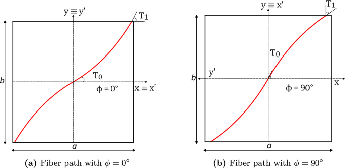
Graphical representation of the parameters involved in a linearly varying fiber path for (left) and (right)
To represent the centerline of the fiber course, one needs to solve the following differential equation:
which, in the case of linearly varying fiber path with and , has the following solution:
Having the equations for the centerline, it is possible to generate the left and right branches of a fiber course at an appropriate distance by incorporating the AFP parameters that emulate the steering process, as illustrated in Fig. 2. A course consists of multiple tows, with the number of tows, , determined by the AFP head’s capacity. Most AFP machines can simultaneously lay down 8, 12, 16, 24, or 32 tows. Given that each tow has a fixed width, , set to 3.125 mm in this document, the total width of a single course, , can be calculated as , being 16 the number of tows considered in this manuscript. Once the AFP manufacturing parameters are established, the various fiber courses for each layer in the laminate are simulated using the geometric parameters depicted in Fig. 2. The expressions for the left and right branches are reported in Eq. (4). Specifically, , , , and represent the x and y coordinates of the left and right branches, respectively, and is the semi-width of the course and is calculated as :
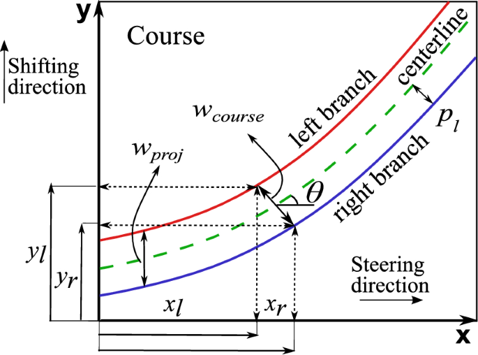
Representation of the AFP parameters that define the centerline and the left and right course branches
The work by Brooks and Martins (2018) established the manufacturing constraints to be considered in optimizing VAT structures. These limitations are related to the AFP machine. The one used in this study is the maximum allowed curvature, which in the case where is calculated as follows:
where denotes the sign function. In this manner, providing a set of and , the local curvature of the fiber path is retrieved and must not exceed the maximum allowed curvature , as shown in Eq. (6), where denotes the minimum turning radius achievable by the AFP machine:
As illustrated in Fig. 2, when examining a generic fiber course, it is evident that the vertical projection of the course width decreases or increases depending on the fiber path angles and . The projected width is calculated as
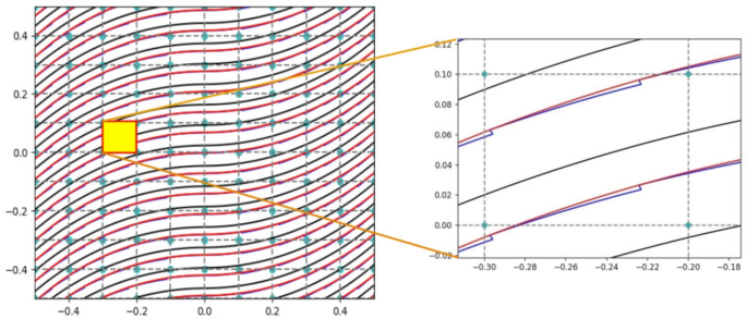
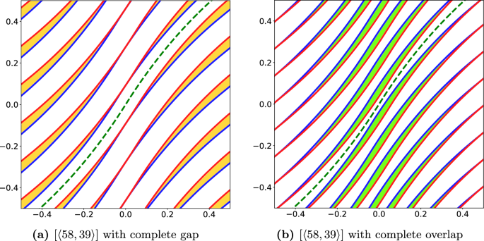
Steering fiber bands along a fixed direction and shifting the AFP head perpendicular to this direction to lay down the consecutive fiber course may result in gaps and/or overlaps. The occurrence of these defects depends on the combination of and angles and the selected deposition strategy, as summarized in Table 1. Two consecutive courses can be set to be tangent at the center or the edge of the plate. In this context, Fig. 3 illustrates the case of a plate, where the tangency condition is applied at the edge and the center. When tangency is enforced at the edge, as seen in Fig. 3a, gaps appear at the center of the plate; conversely, when tangency is imposed at the center, overlaps occur at the plate edges, see Fig. 3b. Similarly, Fig. 4 shows a plate with the same tangency conditions. In this case, the contact-at-the-center strategy results in gaps at the edges, as shown in Fig. 4a, while enforcing tangency at the edges produces overlaps at the center of the plate, see Fig. 4b.
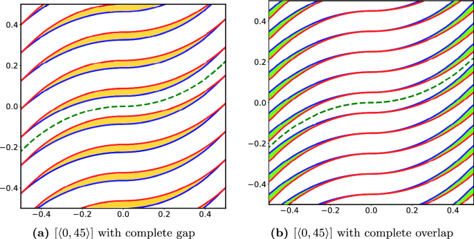
Example of a plate with [] stacking sequence with a complete gap (left) and complete overlap (right) implementing the edge tangency and center tangency steering strategy, respectively. The reference centerline fiber path is shown in green, while the left branch of the course is represented in blue and the right branch in red. Moreover, the gap areas are highlighted in yellow, and the overlap regions in green
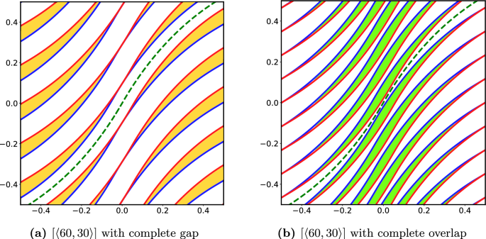
Example of a plate with [] stacking sequence with a complete gap (left) and complete overlap (right) implementing the center tangency and edge tangency steering strategy, respectively. The reference centerline fiber path is shown in green, while the left branch of the course is represented in blue and the right branch in red. Moreover, the gap areas are highlighted in yellow, and the overlap regions in green
A large presence of imperfections is observed in Figs. 3 and 4. It occurs because the width of each course is kept constant during the deposition process. To minimize the defect area, the course width must either decrease when a course intersects with the subsequent one or increase when it does not reach the edge of the previous course. This adjustment in course width is achieved by cutting a single tow and resuming its deposition, resulting in the formation of small triangular defect regions along the fiber path, as shown in Fig. 5. The deposition strategy modeled in this document simulates the correction process with a coverage parameter, establishing the degree of overlap permitted for each course. In particular, only gaps will occur with a coverage value equal to 0%, whereas with a 100% coverage, only overlaps will be generated. Although this work investigates complete gap and complete overlap cases separately, it is worth noting that both defects can coexist within the same lamina. This typically occurs when tows are added or dropped at different stages along the fiber path, leading to mixed triangular gaps and overlap regions. Such situations are naturally described by intermediate values of the coverage parameter, i.e., between 0% and 100%, which result in a combination of the two effects. As shown in the next section, the proposed defect modeling approach is compatible with this condition, as it allows assigning local variations of thickness and material proprieties based on the spatial distribution of defects within each layer.
Representation of the gap defect correction strategy over a [] ply. The zoomed area shows the triangular gaps generated along the fiber’s direction
2.2 Defect layer method
Following the quantification and mapping of the manufacturing defects, it is essential to incorporate them into the structural model via the DLM. The incorporation of defects is accomplished by discretizing the plate’s midplane and modifying the properties of the individual FE depending on the calculated percentage of defects within each FE. In this regard, the only parameter that needs to be changed to simulate the presence of flaws are the material elastic properties or the local thickness. Figure 6 shows the variation of the material elastic properties as a function of the gap area, within the FE, as observed by Fayazbakhsh et al. (2013). The material density varies according to the following rule of mixtures:
in which and are the densities of the pre-impregnated tape and the resin, respectively. In the case of overlaps, the mechanical characteristics of the material are preserved, but the thickness of the FE is locally increased in proportion to the amount of overlap defect, . As stated by Vijayachandran et al. (2020), due to the autoclave compaction pressure, the ply’s maximum thickness increase for this research is limited to 95% as follows:
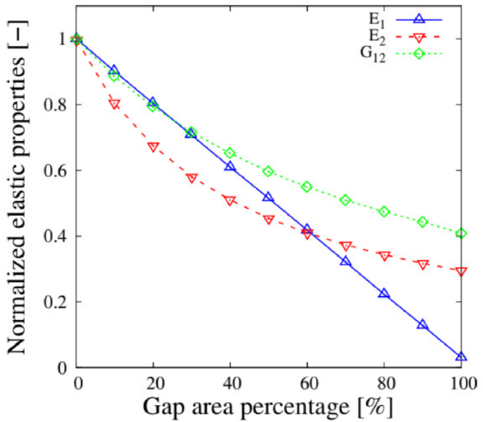
Normalized elastic properties with respect to the gap area percentage. Adapted from Fayazbakhsh et al. (2013) with permission from Elsevier
It can be summarized that when employing DLM for modeling gaps, a multimaterial plate model is generated. In this model, the thickness of each ply is maintained at a constant value and corresponds to that of the defect-free laminate. This enables the straightforward development of LW models through the modification of the material properties of each FE in both the in-plane and thickness directions. In contrast, when modeling overlaps with DLM, the thickness of each FE and layer is not constant but varies spatially. Currently, new methodologies are being explored to develop full LW plates that account for overlaps. Nevertheless, within the context of this research, high-order ESL models are preferable for modeling this particular type of defect. In the case of ESL models, the integration domain along the thickness varies for each FE. Generating an LW model with overlaps represents a complex task because of the required stair-like through-the-thickness discretization. Furthermore, modeling overlaps in an LW framework leads to a notable increase in the degrees of freedom (DOF), which may not provide additional benefits in predicting global structural responses, such as fundamental frequency and buckling load, which are the focus during the presented optimization problems.
3 Structural modeling
This paper implements the CUF framework within 2D FE. According to Carrera et al. (2014), the 3D field of displacements can be expressed as arbitrary through-the-thickness functions of the generalized displacements laying in the plane. This reads as follows:
being M the number of expansion terms. This manuscript employs Taylor expansion (TE) and Lagrange expansion (LE) to generate ESL and LW models, respectively.
TE functions are hierarchical polynomials in the thickness coordinate z. In this approach, the displacement field is expressed as a polynomial expansion in , ensuring a global representation of the through-the-thickness kinematics. A second-order Taylor model is given by
LE functions represent an alternative approach to defining through-the-thickness displacement approximations, particularly in high-order kinematic theories. Unlike Taylor expansions, which use a global polynomial representation, LE discretize the thickness by introducing interpolation points at specific locations. This leads to a subdivision of the thickness into multiple local expansion domains, where the displacement field is approximated using Lagrange polynomials. The polynomial order is determined by the chosen set of interpolation functions. To illustrate this concept, a third-order expansion is provided in Eq. (12):
Usually, to describe the Lagrange functions, it is preferred to use a natural reference system where the variable is defined between and . Equation (13) reports the Lagrange functions related to the third-order expansion:
The choice between TE and LE models depends on the required accuracy and computational efficiency, as TE models provide a global polynomial approximation while LE models allow localized high-order variations in the displacement field. The continuity of the displacements at the layer interfaces is imposed to obtain a Lagrange displacement-based (LD) LW approach, as prescribed in Carrera (2002). In this context, TEn and LDn denote the use of Taylor and Lagrange polynomials of the nth order, respectively. In addition, XLDn is used for LW models to indicate the use of X Lagrange polynomials of nth order per layer. Subsequently, coupling CUF with the FE method, the 3D displacement field is expressed as follows:
where is the number of nodes in the FE, and is the unknowns vector. The present work utilizes bi-quadratic FEs, referred to as Q9, as the shape functions.
The governing equations are derived from the principle of virtual displacements (PVD). The problem is described in terms of virtual work using the principle underlying PVD, which, in the case of free vibration analysis, can be expressed as follows:
where the virtual variation of the internal work, , and the virtual variation of the inertial work, , read as
Equation (16) can be reformulated by employing Eq. (14), the geometrical relations between strains and displacements and the constitutive relations between stresses and strains, resulting in
where is the fundamental nucleus (FN) of the stiffness matrix of the single layer, which is an invariant of the order of the shape function and the theory expansion. Further insight on the FN assembly of ESL and LW models is available later in this section. is the differential operator containing the geometrical relations between strains and displacements, and is the material stiffness matrix defined in the global reference frame. Since this work considers varying fiber paths within the plane, is evaluated point-wise as , being the matrix containing the elastic coefficients of orthotropic material, and is the rotation matrix, as explained in Reddy (2004). Unlike conventional codes, where the fiber orientation is typically assumed constant within each FE, the present implementation evaluates the spatially varying stiffness tensor at the Gauss integration points. This strategy ensures a more accurate representation of the local anisotropic behavior induced by tow steering. In addition, the number of Gauss points can be increased independently of the FE interpolation order, improving integration accuracy without increasing the total number of degrees of freedom. As a result, accurate simulations of VAT laminates can be obtained without resorting to extremely fine meshes since the desired accuracy is achieved by increasing the order of the through-the-thickness expansion functions. A similar approach is applied to Eq. (17), yielding
in which denotes the identity matrix and is the diagonal FN of the mass matrix, as explained in Carrera et al. (2014). The structure’s global mass and stiffness matrices are obtained from their respective FNs based on the shape and expansion functions. These matrices are assembled by looping over the and s expansion indices and the i and j FE indices. Thus, the undamped free vibration problem can be expressed as follows:
where and represent the global mass and stiffness matrices, respectively. The assembly of the stiffness matrix, , depends on the selected modeling approach. The ESL and LW models are frequently employed strategies for analyzing multilayered structures. In the context of ESL modeling, the properties of each layer are homogenized and subsequently combined to compute the stiffness matrix. However, as observed in Carrera (1997), ESL does not satisfy the continuity requirements. In contrast, the LW modeling approach assumes that each layer is treated independently, expanding the displacement field within each lamina. Consequently, displacement continuity must be enforced at each interface (Carrera 2002), ensuring the requirements are satisfied. The two assembly approaches are illustrated in Fig. 7 for a plate with two layers.
Assuming a pure harmonic solution , Eq. (20) results in the following eigenvalue problem:
in which is the natural frequency and represents the eigenvector.
The buckling study consists of solving the equation:
where is the tangent stiffness matrix of the structure. The expression for this matrix is retrieved by linearizing the virtual variation of the internal strain energy:
Substituting Eq. (14), the constitutive law, and the geometrical relations between strains and displacements, the previous equation is rewritten for the case of linearized buckling as follows:
where denotes the FN of the geometric stiffness matrix. This work does not include the explicit equations that allow calculating the tangent stiffness matrix but can be found in Wu et al. (2019). The linearized buckling analysis is performed under the following assumptions: (i) the pre-buckling equilibrium state is stable; (ii) the initial stress remains constant and varies neither in magnitude nor in direction during buckling; (iii) at the bifurcation, the equilibrium states are infinitesimally adjacent so that linearization is possible. At the bifurcation, there exists a critical value of the load factor for which an equilibrium configuration exists where:
In this regard, the buckling load can be computed as , where is the applied load. In Eq. (25), denotes the assembled geometric stiffness matrix of the structure, obtained by looping over the , s, i, and j indices of .
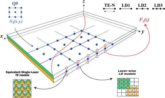
Procedures for assembling ESL and LW plate models
4 Optimization framework
Since the definition of the fiber path of a single ply in a tow-steered composite involves multiple continuous parameters (see Eq. (1)), VAT composites inherently span a much larger, essentially infinite, design space compared to traditional straight-fiber composite laminates. Thus, the design space needs to be explored efficiently to exploit all the possibilities that this kind of structure offers. Besides, if the quantities of interest that aim to be tailored are, a priori, discontinuous, an effective optimization technique must be considered.
This manuscript aims to simultaneously minimize the mass of a VAT plate and maximize a second quantity of interest (QoI), viz., the fundamental frequency or the buckling load. The former depends on the number of plies comprising the laminate, while the latter depends on the fiber path design parameters for a fixed number of layers. Unlike continuous topology optimization frameworks, which optimize material distribution and thickness fields across the design domain (Urso et al. 2023; Urso and Montemurro 2024; Montemurro et al. 2024); this study adopts a discrete approach where the number of plies is treated as an integer-valued parameter while the fiber path parameters remain continuous. Therefore, a mixed-integer, multi-objective optimization problem is faced. In the case that no manufacturing limitations are considered, the optimization problem is stated as follows:
in which is the number of layers for each design, varying between the lower and upper bound, and and are the vectors containing the individual and angles for each layer of the current design. To reduce the number of design variables and ensure practical stacking sequences, symmetry, and quasi-symmetry were enforced a priori. Symmetric laminates were used when is even, while quasi-symmetric configurations were adopted for odd-layered designs.
The solutions to the unconstrained multi-objective could not be feasible from a manufacturing perspective. Therefore, manufacturing limitations must be considered. As anticipated in Sect. 2, the main constraint considered is the AFP head’s turning radius. This is a constraint that needs to be fulfilled for each layer in the laminate. In this context, the constrained multi-objective optimization problem can be posed as follows:
where the manufacturing constraint is aggregated through a product of a maximum value operator over the number of layers in the design. The operator chooses between 1 and the ratio . In this regard, if the curvature constraint is satisfied for all the plies, the product will equal 1. This formulation ensures that if a single layer exceeds the permissible curvature, the collective constraint will be violated, thereby steering the optimizer away from inherently infeasible designs. Using the product operator, the optimization solver can identify how far the evaluated design is from fulfilling the manufacturing constraint for all the plies in the design.
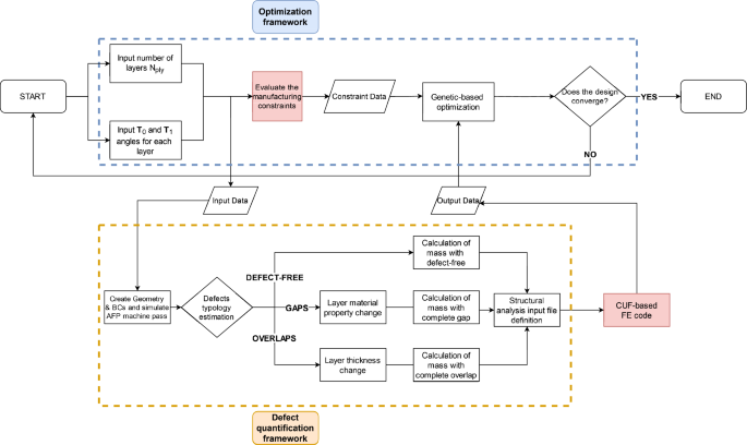
Flowchart of the multi-objective mixed-integer optimization framework considering the manufacturing constraint and the quantification of the defects performed by DLM. Finally, the CUF-based FE code is used to calculate the fundamental frequency and buckling load
In this study, the non-dominated sorting genetic algorithm II (NSGA-II) (Deb 2001), incorporated in modeFrontier©(Nardin et al. 2009), is employed to address the mixed-integer, multi-objective optimization problem associated with VAT laminates. NSGA-II is particularly well-suited for this application due to its robustness in handling complex design spaces that combine discrete and continuous variables (Jaber et al. 2021), as required here to simultaneously optimize the number of laminate plies and fiber orientation angles. Unlike traditional gradient-based optimization methods, NSGA-II does not require derivative information, making it highly effective for the inherently discontinuous, multi-modal design space of VAT laminates (Montemurro and Catapano 2016). The algorithm’s non-dominated sorting and crowding distance mechanisms are crucial for identifying a diverse set of optimal solutions across the Pareto front, balancing mass minimization with performance maximization (regarding fundamental frequency and buckling load). Moreover, NSGA-II’s elitist approach ensures that the best solutions in each generation are retained, accelerating convergence towards the Pareto-optimal front. This feature is vital for optimization problems like the one in this study, where manufacturing constraints such as the AFP head turning radius impose strict limits on feasible fiber paths. These enhancements, implemented within the NSGA-II framework, are particularly suited to addressing the complexities of mixed-integer optimization in VSC design. They enable efficient exploration of the high-dimensional design space while ensuring computational feasibility, as demonstrated by Jaber et al. (2021). Utilizing the product-based aggregation form of the optimization constraint, as seen in Eq. (27), within the NSGA-II framework guides the algorithm away from infeasible designs by evaluating curvature compliance collectively across all layers, rather than filtering each layer individually. This approach allows NSGA-II to focus effectively on feasible regions of the design space.
A key aspect of this optimization strategy is the synergy between NSGA-II and the DLM, explained in Sect. 2, which is incorporated to quantify manufacturing defects in the numerical model. The DLM operates in conjunction with NSGA-II, providing accurate defect quantification for each evaluated design, which is crucial for a realistic assessment of VAT performance. Figure 8 illustrates the optimization workflow of the constrained problem. In the case of the unconstrained optimization, the check on the manufacturing constraint is skipped. First, an initial set of individuals is generated, whose design variables are the number of layers in the laminate and the fiber path angles. Subsequently, based on the different and , the maximum curvature of the fiber path is calculated. Then, the input data of the FE analysis is generated. Only the number of expansion domains and the fiber angle orientation are modified if the defect-free condition is considered. Otherwise, if a complete gap or overlap condition is preferred, the material and thickness of each FE are modified according to the DLM. In addition, depending on the fabrication strategy, the mass of the plate is calculated as
where is the homogenized density associated with the gap-defective FE, which is computed through the rule of mixtures, is the thickness associated with the overlap-defective FE, calculated according to Eq. (9), and is the number of FE in the numerical model. Then, the FE simulation is launched, and the value of the fundamental frequency or buckling load is retrieved. Last, the genetic operations are performed until convergence of the Pareto front is reached.
5 Numerical results
5.1 Defect modeling verification
The defect-mapping procedure depicted in Sect. 2 is verified against the results present in the work by Akbarzadeh et al. (2014) for fundamental frequency and buckling load. The structure under investigation is a 16-layered symmetric and balanced laminate and width-to-thickness ratio . The width and length of the plate are m, and the individual ply thickness equals 0.159 mm. The plate is simply supported on all four sides. The mechanical properties of the pre-impregnated tows and the resin are listed in Table 2. The reference plate is illustrated in Fig. 9. In particular, Fig. 9a depicts gaps at the edges, while Fig. 9b illustrates the presence of overlaps in the central area.
Reference plate from Akbarzadeh et al. (2014) with [] stacking sequence with a complete gap (left) and complete overlap (right) implementing the center tangency and edge tangency steering strategy, respectively
The effect of the structural theory is addressed in the presence of manufacturing signature after performing a convergence analysis on the number of FE. In the case of fundamental frequency verification, a mesh is employed because of the trade-off between accuracy and computational time. Gap-defective plates are modeled through ESL and LW models. In contrast, overlap-defective plates are modeled only with ESL models due to the high computational cost of modeling overlaps with an LW approach, as explained in Sect. 2. Table 3 shows the first fundamental frequency results for the complete gap and complete overlap strategies. Although there is a good agreement between the proposed methodology and the reference solution, there exist slight differences. The reasons are twofold: (i) the reference solution employs Reddy (2004) third-order shear deformation theory, which assumes a constant displacement component while the present method foresees high-order terms for the three displacement components; and (ii) the reference values are obtained through a semi-analytical approach employing the Galerkin method and Fourier series expansion to solve the governing differential equations, whereas the present work employs a fully numerical method. In addition, it is found that, in the case of complete gap strategy, there is no significant difference between ESL and LW models in terms of the predicted . In the case of complete overlap, there is no meaningful difference as the order of TE increases.
The defect-mapping procedure is then verified to predict the buckling load of VAT plates in the presence of defects. The laminated structure described above is now subject to an in-plane shortening at . The dimensionless buckling loads predicted by the various structural theories are displayed in Table 4. A mesh is utilized because of the accuracy and computational time trade-off. A good correlation is found between the present results and the reference, with the differences lower than the first fundamental frequency case. The reasons for the discrepancies have been mentioned above, i.e., the reference’s structural theory and solution approach. Regarding the present structural models, ESL and LW theories lead to similar values of dimensionless buckling load when the complete gap strategy is chosen. In the case of complete overlap, the ESL-TE 1 model presents the largest value of compared to higher order ESL theories. In any case, the differences in results between the modeling strategies are minimal because of the large width-to-thickness ratio of the plate under study. If a thicker plate were analyzed, the shear stress components would be more relevant, and higher order models would be required.
5.2 Least-weight design optimization
5.2.1 Mass versus fundamental frequency optimization
The first least-weight problem combines minimizing a laminated plate’s mass and maximizing its fundamental frequency. The AFP machine’s manufacturing signature and strategy are included in the optimization loop following the procedure depicted in Sect. 4. The plate under investigation has a width and length m and a ply thickness of 0.159 mm and is fully clamped. The material properties are available in Table 5.
The optimization results are compared against the optimal straight-fiber case reported in Carvalho et al. (2022). This work only considered the fundamental frequency as the objective function. The number of plies was fixed to eight, and symmetry was imposed a priori for the laminate stacking sequence. The present work considers symmetric laminates to reduce the number of design variables. The optimal solution by Carvalho et al. (2022) presents a lamination, a fundamental frequency equal to 54.68 Hz, evaluated with the FEM implemented in the present work and the mesh, and a mass of 0.5247 kg.
Figure 10b displays the Pareto fronts of the defect-free manufacturing strategy and different structural theories for the unconstrained and manufacture-constrained problems. The optimization constraint is set equal to 3.28 m. Table 6 provides the stacking sequence for the seven-layered non-dominated design, while Fig. 11 illustrates the optimal fiber paths in the defect-free scenario utilizing the LW-LD2 structural theory for both unconstrained and constrained solutions. For the mass versus fundamental frequency optimization case, it was decided to represent the fiber paths of only half of the laminate, as the structure is symmetric. The complete gap Pareto fronts are depicted in Fig. 12, and the corresponding seven-layered designs are presented in Table 7. The optimal symmetrical fiber paths for the LW-LD2 model, determined under the specified manufacturing conditions, are illustrated in Fig. 13. Finally, the Pareto front for the complete overlap strategy is presented in Fig. 14, with the corresponding symmetrical six-layered overlap designs detailed in Table 8. The optimal fiber paths for the ESL-TE3 model under the complete overlap strategy are depicted in Fig. 15. It is worth noting that the green dots in the Pareto fronts correspond to all the designs evaluated during the optimization process utilizing the LW-LD2 structural model for defect-free and complete gap manufacturing strategies. In the complete overlap Pareto fronts, the green dots correspond to the ESL-TE3 designs. The designs of the low-order ESL theories are not represented for the sake of clearness.
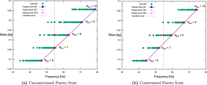
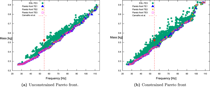
Defect-free Pareto fronts for the mass versus fundamental frequency optimization, illustrating the (a) unconstrained and (b) constrained cases. The results are derived using ESL and LW models to reflect the influence of different structural theories
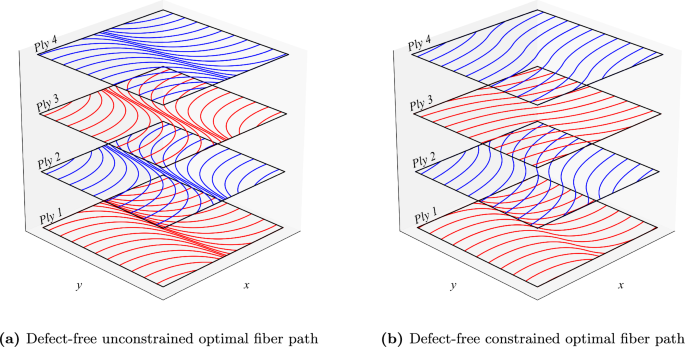
Defect-free unconstrained and constrained optimal fiber paths using LW-LD2 structural theory, shown for half of the laminate due to its quasi-symmetric configuration
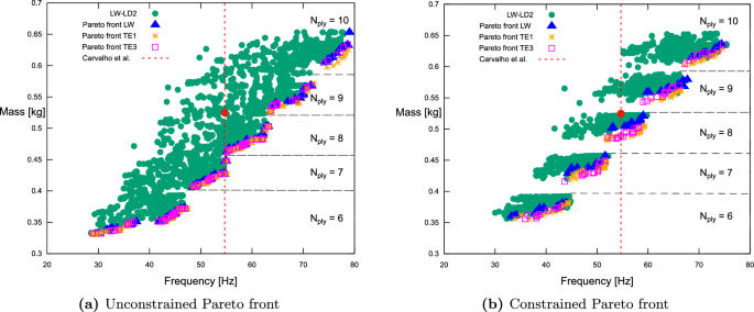
Complete gap Pareto fronts for the mass versus fundamental frequency optimization, illustrating the (a) unconstrained and (b) constrained cases. The results are derived using ESL and LW models to account for the influence of the structural theory
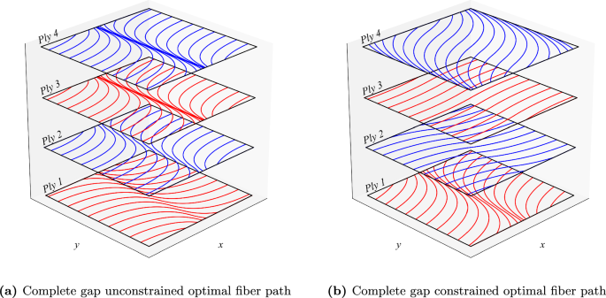
Complete gap unconstrained and constrained optimal fiber paths using LW-LD2 structural theory, shown for half of the laminate due to its quasi-symmetric configuration
Complete overlap Pareto fronts for the mass versus fundamental frequency optimization, illustrating the (a) unconstrained and (b) constrained cases. The results are derived using high-order ESL models to capture the influence of the structural theory
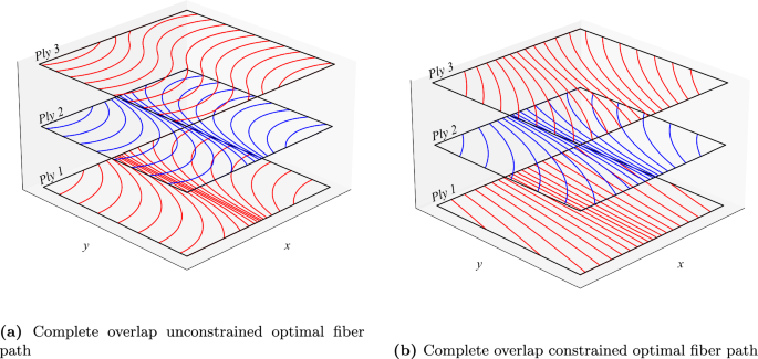
Complete overlap unconstrained and constrained optimal fiber paths using ESL-TE3 structural theory, shown for half of the laminate due to its symmetric configuration
From the results outlined, the following comments can be made:
- The discrete nature of the optimization problem is highlighted in the defect-free and complete gap manufacturing strategies. The former presents a constant mass for each ply while the fundamental frequency varies. The latter exhibits a scattered set of designs, where the mass and fundamental frequency vary, even when the number of layers is kept constant. These banded sets are better appreciated in the complete gap-constrained Pareto front in Fig. 12b, which are due to the density associated with each FE, as depicted in Eq. (28). These banded fronts do not exist in the complete overlap optimization results, in which the parameter varying the mass for a fixed number of plies is the thickness associated with each FE.
- There is a weak influence of the structural theory on the defect-free case’s unconstrained and constrained Pareto fronts. This is further observed in Table 6, where the only discrepancy occurs for in the constrained case.
- A slight variability is observed in the Pareto fronts corresponding to the complete gap and overlap strategies, as shown in Figs. 12 and 14, respectively. This variation becomes more pronounced as the number of plies increases and is attributable to the different structural models employed. Despite this, the optimal fiber path for the first layer, , remains consistent across manufacturing strategies and structural theories for both the constrained and unconstrained cases, with the only exception being the constrained ESL-TE1 complete overlap solution. It is worth noting that the ESL-TE1 model, which resembles FSDT formulations commonly used in commercial software, exhibits limitations in accurately capturing transverse shear effects.
- The outermost layers dominate in bending problems like the first free vibration mode, while the innermost plies are dominated by shear components. In this regard, only high-order models can predict these shear components accurately and, ultimately, provide better optimal designs for the innermost layers. This is observed in the optimal results for the three manufacturing conditions, structural theories, and the unconstrained and constrained optimization problems investigated.
- For unconstrained optimizations, when defects are not considered, results show that a seven-layer VAT plate can achieve designs with fundamental frequencies equal to or higher than the optimal eight-layer straight-fiber baseline. Even when a complete gap strategy is applied, seven layers are sufficient to reach at least the optimal frequency of the straight-fiber laminate. Weight savings for these configurations range from 12.5% in the defect-free solution to 18.5% with the complete gap solution. Consequently, Figs. 11a and 13a display the optimal fiber orientations for the first four layers of the quasi-symmetrical laminate. In contrast, only six layers are needed for the complete overlap condition to achieve a natural frequency higher than the eight-layer straight-fiber reference, resulting in a 19.5% weight reduction. Figure 15a illustrates the optimal fiber orientations for the first three layers of this symmetrical laminate.
- When the constraint on fiber path curvature is applied, the complete overlap strategy is the only approach that enables a six-layer VAT plate to achieve a fundamental frequency higher than the eight-layer straight-fiber one. The fiber paths for the first three layers of this optimal symmetrical laminate are shown in Fig. 15b. In contrast, if defects are neglected or the complete gap strategy is used, eight layers are needed to reach a fundamental frequency above the baseline of 54.68 Hz. The optimum results for the seven-layer configuration are reported in Table 6 for the defect-free case and in Table 7 for the complete gap case to highlight the mass reduction relative to the reference case while maintaining a natural frequency below the baseline. Figures 11b and 13b show the optimal fiber trajectories for the first four layers in the defect-free and complete gap scenarios, respectively.