Article Content
1 Introduction
Due to the high manufacturing flexibility offered by Additive Manufacturing, Multi-Material Topology Optimization (MMTO) of lattice structures has received considerable momentum in recent research. The main challenge in MMTO is to perform it without significantly increasing the cost of renewing the design variables, which is mainly related to the number of used materials and can be controlled using proper material interpolation.
In the density-based approach, also known as the SIMP (Solid Isotropic Material with Penalization) method (Bendsøe 1989; Zhou and Rozvany 1991), Topology Optimization (TO) is conducted by first placing the two candidate materials (void and solid) over the vertices of a line interpolation domain (), typically void (white) at and solid (black) at . In this paper, the term “interpolation domain” refers to the domain of definition of the interpolation function. To avert solving such a 0–1 binary optimization problem, a non-physical transitory phase (gray) between void and solid is introduced, which should also be made less effective by use of a penalized interpolation of the elements stiffness such as the modified power-law (Andreassen et al. 2010)
Here, is a vector that contains the pseudo densities of the N finite elements; is the Young’s modulus for the used material; is a small positive number to avoid singularity; and is a penalization factor. Equation (1) might also be solved without the relaxation-penalization scheme as in Sivapuram and Picelli (2017), Liang and Cheng (2019) and Liang et al. (2020).
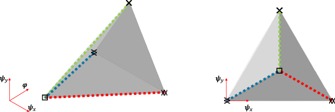
In MMTO, the SIMP method could be extended to account for three or four materials by replacing the 1D line interpolation domain by 2D square or 3D cube interpolation domains, respectively, and similarly placing the candidate materials over the corresponding vertices as illustrated in Fig. 1(top). Then, the power-laws for interpolating three and four materials read (Bendsøe and Sigmund 2004)
respectively, where are the three design variables; and are the Young’s modulus for the first, second, and third materials, respectively. Further extensions to include materials is theoretically possible by using an -D hypercube interpolation domain. However, the usage of the extended SIMP method in the literature is limited to three and four candidate materials (including void) (Gibiansky and Sigmund 2000; Taheri and Suresh 2016; Gaynor et al. 2014; Gao and Zhang 2011), as a study by Stegmann and Lund (2005) showed that including more than four candidate materials tends to converge to bad local minima.
An alternative method that is capable for handling higher numbers of candidate materials is the Discrete Material Optimization (DMO) (Stegmann and Lund 2005), which illustrated capabilities for optimizing the orientation of composite laminate based on an orthotropic material with 12 different angles (Stegmann and Lund 2005; Lund and Stegmann 2004), as well as material selection problems with 6 (Sanders et al. 2018a) and up to 15 (Sanders et al. 2018b) candidate materials. This method expresses the element elasticity tensor as a weighted sum of the elasticity tensors of all candidate materials (Stegmann and Lund 2005). Similarly, the vector contains the isotropic properties for the N mesh elements interpolated as
where are the weights defined as
As seen in Eq. (3), the DMO method, unlike the extended SIMP method (Eq. (2)), does not explicitly consider void as a candidate material, as zero-stiffness appears when all design variables are zero or when more than one design variable equals 1. However, the two methods require using an -D orthogonal material interpolation domain, but with a slightly different material placement as compared in Fig. 1.
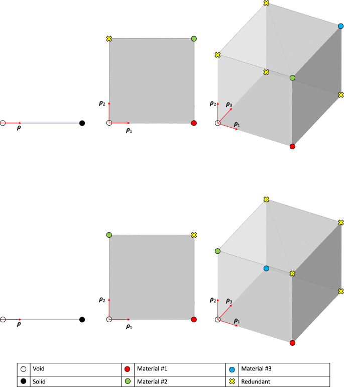
Orthogonal material interpolation domains used in the SIMP (top) and DMO (bottom) interpolation schemes for accommodating two (left), three (middle), and four (right) candidate materials
It is not that simple to determine whether the DMO method or extended SIMP method is better than the other. For instance, a study done by Gao and Zhang (2011) showed that DMO converges to better local minima than extended SIMP, even when only three candidate materials are used. On the other hand, the study of Liu et al. (2023) demonstrated that a discrete formulation of the extended SIMP method can effectively solve MMTO problems as Eq. (2) has separable characteristics in sensitivity analysis of discrete variables in comparison to Eq. (3).
Furthermore, the study of Yi et al. (2023), proposes a unified material interpolation method that follows the DMO material placement [Fig. 1(bottom)], but with an alternative mapping based on the p-norm of the design variables in order to model each material equally. The method showed clear convergence to 0–1 solution for each material in comparison to both DMO and extended SIMP. Similarly, Huang and Li (2021) obtained clear 0–1 designs using an interpolation method based on the physical volume fractions of candidate materials within each element.
To sum up, the most common thing between the extended SIMP, DMO methods, unified material interpolation, and other multivariate methods, is the need for design variables per mesh element e. This makes the memory cost of renewing the total design variables higher with increasing the number of candidate materials, especially when optimizing Functionally Graded Lattices (FGL) where the number of candidate materials (lattices) easily exceeds ten.
This led to another approach that decouples the dimensionality of the interpolation domains from the number of candidate materials. For instance, the Shape Functions with Penalization (SPF) scheme proposed by Bruyneel (2011) employs the conventional bi-linear shape function of the first-order quadrangular finite element for interpolating between four candidate materials placed over the vertices of a 2D square domain, which resulted in using only two design variables instead of four. According to the author, this could also be extended to include up to seven candidate materials and stay in 2D space by using shape functions with mixed degrees on the edges. However, for including more than seven candidate materials, considering a 3D cube domain would be recommended. Figure 2 shows the interpolation domain and material placement used with SFP.
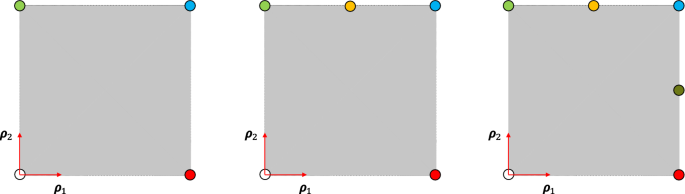
Square material interpolation domain used in the SFP interpolation scheme for accommodating four candidate materials (left) and possible formulations for accommodating five (middle), and six (right) candidate materials
The dimensionality of the interpolation domain could be further reduced by using univariate interpolation methods which use only one design variable per mesh element regardless of the number of used materials. In this approach, the candidate materials are placed over a 1D line interpolation domain , according to their normalized densities , and then the properties between each two adjacent materials, for instance and , are interpolated by a continuous function, as illustrated in Fig. 3.
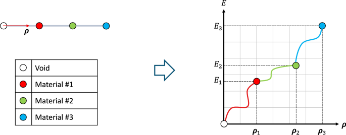
Four candidate materials sorted over a line interpolation domain according to their densities (left) and the corresponding interpolated property between each two materials (right)
In the literature, a wide variety of continuous functions are used to describe the transitions between the candidate materials (i.e., the red, green, and blue lines in Fig. 3(right)). For instance, the researchers used a straight line (Liu et al. 2021), SIMP power-law (Zuo and Saitou 2016; Augusto and Palma 2022; Nguyen and Lee 2024), SIMP-like power-law (Xu et al. 2021), peak function (Yin and Ananthasuresh 2001), stair-form function (Liao et al. 2024), Heaviside function (Liao 2021; Jiang et al. 2024), and smoothened Heaviside function (Dinh et al. 2024). In addition, multi-valued integer programming is also used to solve multi-material optimization problems without the relaxation-penalization approach (Deng et al. 2024).
The candidate materials could also be sorted based on other physical properties, such as Young’s modulus. This would be very useful in case of using candidate materials with similar or close densities, as in Guo et al. (2024) and Wan et al. (2024), and when optimizing FGL, where it is practical to decouple between the solid-void phases and the candidate lattices by using two distinct interpolation domains and bridge them by the Porous Anisotropic Material with Penalization (PAMP) method (Liu et al. 2008), as illustrated in Fig. 4. On the one hand, and as presented before, the void and solid phases are typically placed over the vertices of a line domain and interpolated through the SIMP power-law (Eq. (1)). On the other hand, for interpolating between the lattices, the designers have more freedom in choosing the interpolation domain and interpolation function (f). In the two following paragraphs, we discuss them in more details.
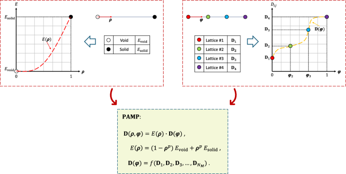
Two distinct line interpolation domains used for accommodating the solid-void phases (top left) and four lattices (top right), and then bridged by the PAMP method (bottom)
How to choose the interpolation domain ? In the simple case of using one family of FGL (i.e., a group sharing similar geometrical features), as in Wang et al. (2018, 2020a), employing a line interpolation domain is sufficient. However, when more families (having different densities or different geometrical features, for instance) are considered, the 1D line interpolation domain is typically extended orthogonally (as in Fig. 1) to 2D square (Costa et al. 2022; Wang et al. 2020b, 2023), 3D cube (Zhang et al. 2023; Yang et al. 2024), 4D hypercube (Zhang et al. 2022; Zhou et al. 2022), or higher. To the best of our knowledge, using custom-designed non-orthogonal domains in TO of FGL have not yet been studied. As these domains require additional processes, such as treating the strayed design points (i.e., points goes outside the domain), they also eliminate the existence of redundant entries seen in Fig. 1 as we suggest that the permutation of the families affects the optimization process and may promote bad local minima. Alternatively, motivated by the study of using a diamond interpolation domain in designing a multiphase electrical machine’s stator (Cherrière, Théodore et al. 2022), we propose using equilateral non-orthogonal domains as they provide equal distances between any two families, and more importantly, there is no need to duplicate some families to fill the redundant edges. Examples of accommodating three families of FGL in cube and triangular prism domains are given in Fig. 5.
Three families of FGL (top) accommodated in orthogonal (bottom left) and non-orthogonal (bottom right) interpolation domains
How to choose the interpolation function (f)? For instance, the polynomial fitting method is very simple and provides continuous derivatives. Depending on the definition of the selection parameter , the fitting degree could be chosen as 2 (Zhang et al. 2022, 2023), 3 (Wang et al. 2018; Yang et al. 2024), or 5 (Wang et al. 2020a, b; Costa et al. 2022). Another alternative method that exhibits local penalization to push more toward the candidate lattices is the ordered SIMP (Zuo and Saitou 2016; Augusto and Palma 2022) and applied in Zhang et al. (2018) and Gu et al. (2022). Furthermore, a recent method with both local penalization and continuous derivatives has been proposed by Dinh et al. (2024) but not yet employed in TO of FGL. In this paper, we study, on the one hand, the effect of using custom-designed material interpolation domains for accommodating three families of FGL. Our compared domains include 2D and 3D, as well as orthogonal and non-orthogonal ones. On the other hand, we also study replacing the classical polynomial fitting method with some advanced methods that offer local penalization and smoothening, namely the ordered SIMP (Zuo and Saitou 2016; Augusto and Palma 2022) and smooth single-variable interpolation (Dinh et al. 2024). One of the novelties of our paper is that we use the concept of Coons patches (Coons 1967) to extend the univariate methods to 2D and 3D domains and use only two and three design variables, respectively, regardless of the number of used lattices.
The rest of this paper is structured as follows. In Sect. 2, we formulate our topology optimization problem and describe the technique used in solving it. Then, the studied interpolation domains and interpolation functions are introduced in Sect. 3. After that, in Sect. 4, the optimization problem and the results are presented and discussed. Finally, we conclude the comparison in Sect. 5.
2 Topology optimization formulation
In this section, we first introduce our materials and design variables. Then, we define our optimization problem and describe the technique used to solve it.
2.1 Materials and their properties
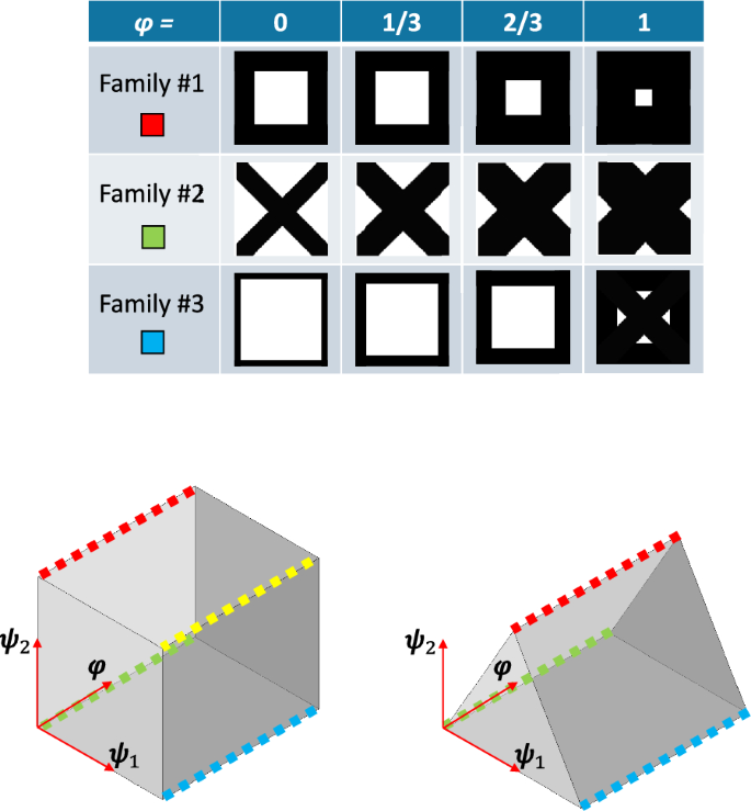
In this study, we use 28 lattices (orthotropic materials), which were developed in a previous work (Ali et al. 2024). These lattices have identical costs and weights and are grouped into three families according to their geometries. For navigating between the lattices, in the previous work, we used the design variables and to indicate the family (row) and lattice (column), respectively, as shown in Fig. 6(top). In this study, we investigate alternative ways as follows in Sect. 3.1.
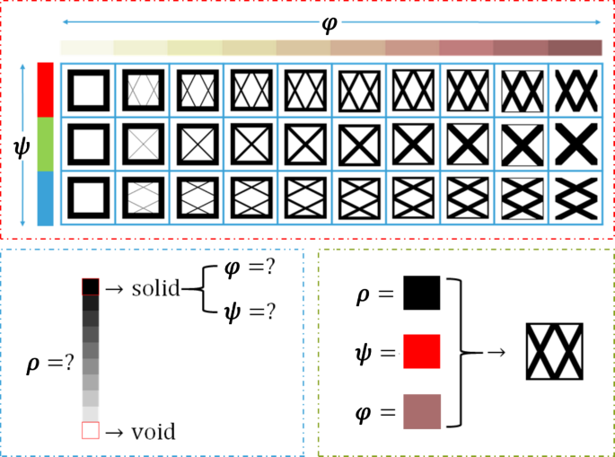
Lattices grouped in three families (top), design variables (bottom left), and an illustration for selecting the material (bottom right)
The stiffness of each mesh element e is calculated, using the Porous Anisotropic Material with Penalization (PAMP) method (Liu et al. 2008), as
where is the pseudo density used to distinguish between solid and void. The first component depends on the pseudo density and is obtained by using the modified SIMP method (Sigmund 2007) via
where p is a penalty factor; is Young’s modulus of the isotropic material; is a very small positive number to prevent the singularity of the stiffness matrix. Here, we typically use , , and .
The second component depends on the material and is evaluated through numerical homogenization (Andreassen and Andreasen 2014)
where is the (i, j)-th component of the homogenized elasticity tensor for ; and are the domain and volume of the element e, respectively; M is the total number of micro-elements; is the element displacement solution corresponding to the unit strain field which is , , and for , and 6, respectively; The superscript indicates the micro-scale and is the stiffness matrix for the micro-element , calculated as
with as the strain–displacement matrix; and
and
where and are the Young’s modulus and Poisson’s ratio for the base material. Here, we assume plane-stress state and choose , which captures well the geometrical features of our micro-structures and satisfies the assumption of length-scale separation, i.e., the micro-structures are much smaller than the macro-structures. We also take and . The obtained equivalent moduli of the lattices are plotted in Fig. 7.
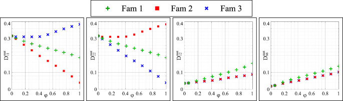
Effective elastic moduli for the lattices
2.2 Optimization problem
Since the density and cost of our materials are the same, they will not be considered in our density-based topology optimization formulation. With the objective of minimizing structural compliance and constraining the volume, our optimization problem can be formulated as follows: Minimize
such that
and
where C is the structural compliance; is the stiffness matrix; and are the displacement and force vector, respectively; is the first inequality constraint and represents the material volume ( and are used in Sect. 3.1 and illustrated in Fig. 12); is the maximum allowed volume fraction; and is an interpolation domain and should not be confused with the design domain . The former is used to accommodate the candidate materials (Figs. 1, 3, and 5), while the latter represents the allowable space where material can be added or removed during the optimization. It is worth mentioning that the dimensionality of the interpolation domain and design domain are not linked at all. For instance, a 1D interpolation domain could be used in optimizing 2D or 3D structures. Further details about interpolation domains are given in Sect. 3.1.
The sensitivities of the objective and constraint functions were derived in Ali et al. (2024). For the sake of brevity, we directly present the final formulas, which are given as
where is the strain–displacement matrix; and the terms and are the gradients of the interpolating functions presented in Sec. 3.2. The term is obtained directly from Eq. (5) via
2.3 Optimization algorithm
At the beginning of the optimization process, we set all the design variables to the centroids of the considered interpolation domain, and then update all of them concurrently. The optimization is conducted using the Method of Moving Asymptotes (MMA) (Deetman 2019) and is repeated until the improvement in the compliance is less than 0.1% for ten successive iterations. To prevent the checkerboard problem, is filtered by using the sensitivity filter (Sigmund 1997), while the density filter (Bourdin 2001) is applied for filtering and . In all cases, the minimum filter radius is set to , i.e., to two mesh elements.
3 Material interpolation schemes
In this study, we concentrate on two aspects of multi-material modeling: which interpolation domains should be used and how the relation between our materials should be described. We explore several possibilities to answer these two questions in the following subsections.
3.1 Interpolation domains
How we place (arrange) our materials depends on the shape of the selected interpolation domain. We denote by the interpolation domain, which is a convex polytope containing the admissible interpolation variables . Generally, the candidate materials are placed over nodes inside the domain (see Figs. 9, 10, 11, and 13), so that when an interpolation variable is equal to a node coordinate, it designates a “real” candidate material. Otherwise, it is associated with a “gray” intermediate material. In classical void/solid topology optimization, the only possible interpolation domain is a segment with only two vertices, while in MMTO, many interpolation domains are possible. The choice of affects the optimization progress and may lead to convergence to a bad local minimum.
In this work, we aim to compare 2D and 3D interpolation domains, as well as orthogonal and non-orthogonal domains. The main advantage of using orthogonal domains is the ease of keeping the design points inside the domain (i.e., ) by means of box constraints with the following projection operator:
where is the orthogonal projection operator onto an orthogonal domain; is an optimization variable (for instance, or ) lying between two bounds and . It is worth mentioning that Eq. (12) is already developed in the MMA solver, and one only needs to define the parameters and , according to the bounds of the interpolation domain.
On the other hand, using non-orthogonal domains gives more freedom in setting the number of edges and vertices but requires a more complicated projection technique. The selected domains are illustrated in Fig. 8 and are introduced below.
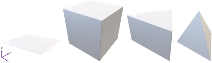
Interpolation domains (from left to right): Square, cube, triangular prism, and triangular pyramid
3.1.1 Square domain
A square domain is the classical orthogonal domain in 2D. We set its size to and divide it into subdomains in the directions of and , respectively. We then place our materials over the 30 nodes according to their values (plotted in Fig. 7), as illustrated in Fig. 9. However, a potential major drawback is the lack of connections between the families, i.e., the resulting interpolation is not necessarily monotone. For instance, it is not possible to go from the red family (at the bottom) to the blue family (at the top) without going through the green family (at the middle), which could result in converging to a bad local minimum.
It is worth mentioning that sorting the families according to their values does not affect the optimization process significantly since the curves of and are reciprocated for Family #2 and Family #3 and same for Family #1. However, sorting the families according to the curves of or negatively affects the optimization process. This is probably because Family #2 and Family #3 have identical curves for and for , and when we place them beside each other, we create regions of almost zero-slope and negatively affecting our gradient-based optimization.
On the other hand, sorting the lattices inside each family also affects the optimization progress and the order should be chosen wisely. For instance, sorting the lattices (changing the definition of in the horizontal axes in Fig. 7) in an ascending or descending order would be the best choice. However, choosing a U-shaped or bell-shaped order gives similar results, but have high sensitivity to initial guess and is not recommended.
Square domain: material placement
3.1.2 Cube domain
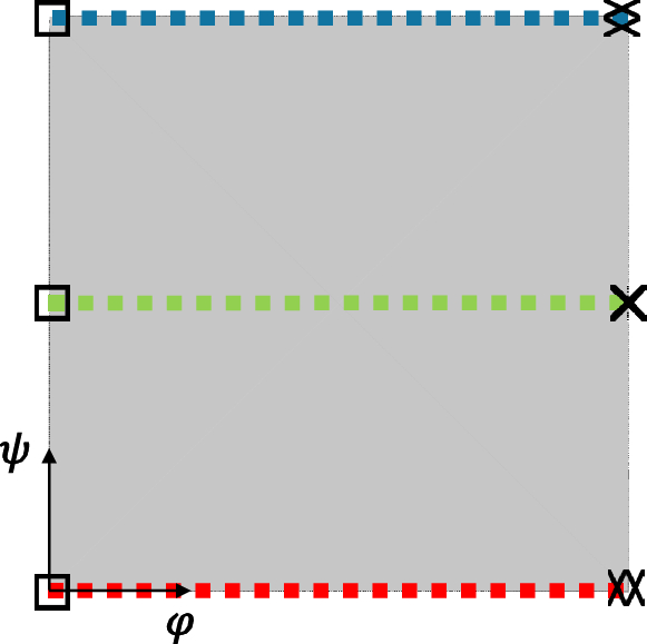
The primary motivation for using a cube domain is to overcome the connectivity issue in the square domain. We take a cube of size and place the families over the edges parallel to the -axis as illustrated in Fig. 10(bottom). In the remaining fourth edge, we examine the four possibilities shown in Fig. 10(top). Case I, II, and IV are inspired by the DMO, extended SIMP, and SFP methods (Figs. 1 and 2), respectively, with the black circle representing an artificial family (family #0) that contains only voids.
Since this domain and the following domains are 3D, becomes, from now on, a vector with components in x and y.
Cube domain: Studied family placements (top) and material placement for Case I (bottom)
3.1.3 Triangular prism
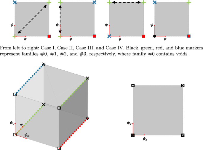
A further improvement compared to the cube domain is achieved using a non-orthogonal triangular prism domain, eliminating the need to duplicate a family or introduce a redundant one. We consider a uniform right triangular prism, cf. Fig. 11. The coordinates of the base triangles are (0, 0, 0), (1, 0, 0), and and the height of the prism is 1.
During the optimization process, some design points may go outside of the prism, for example, to the coordinate . In order to prevent this, we project the strayed points back to the non-orthogonal domain after each iteration. Since the MMA’s box constraints (Eq. (12)) are not enough, from now on, we apply an angular projection, which is illustrated in Fig. 12a. It is worth mentioning that turning off the box constraints did not affect the results. In addition, other more expensive techniques like orthogonal projection or incorporating linear constraints into the optimization process, see Fig. 12b–c, resulted in very similar designs.
Triangular prism and material placement
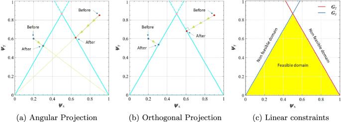
Techniques for updating design variables within a triangular domain
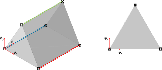
3.1.4 Triangular pyramid
As seen in Figs. 6 and 7, the three families are identical at and become more distinct by increasing . This phenomenon makes the replacement of the triangular prism by a triangular pyramid more realistic. Besides, the square-shaped lattice () does not have to be replicated three times as in the previous domains. Accordingly, we include a triangular pyramid domain with vertices located at , (0, 0, 1), (1, 0, 1), and . To avoid singularity issues, the tip node of the pyramid, i.e., point , is replaced by a very small triangle between points , , , with . Through this modification, the pyramid domain becomes a frustum (prism), which can be mathematically handled as the prism domain before. The domain and the material placement are visualized in Fig. 13.
Triangular pyramid
3.2 Interpolation functions
After deciding how to arrange our materials, the second question is how to interpolate between them. In this section, we compare different interpolation methods like the classical polynomial fitting, ordered SIMP, and smooth single-variable-based interpolation for interpolating and its derivatives and in Eqs. (8), (9) and (10). Figure 14 gives a general overview of the methods, further presented in the following subsections.
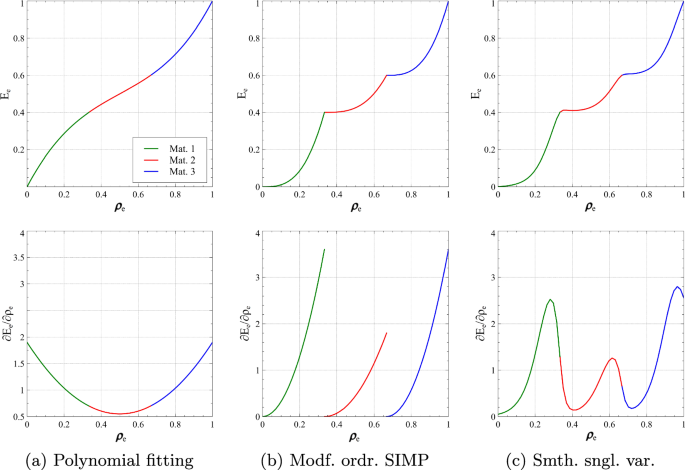
Interpolation functions (top) and their first derivatives (bottom) with and (
We start with introducing the methods used to interpolate the stiffness of isotropic materials with respect to pseudo density, i.e., in 1D domains. Here, we interpolate each scalar component of the stiffness matrices of our orthotropic materials with respect to geometry design variables, i.e., and also extend the methods to 2D and 3D domains.
3.2.1 Polynomial fitting
This classical method is featured by its continuous function and derivatives; see Fig. 14a. It approximates the modulus as
where are the fitting coefficients; and n is the fitting degree. Here, we have two directions to fit. In the direction of , we choose n such that all families are interpolated, i.e., the coefficient of determination equals one, which means for the square domain and for the other ones. In the direction of , we set , which results in good fittings with all .
This method is not favored in MMTO due to its lack of penalization, which means the optimized design will have very scattered design points (non-physical material points) rather than converging to the predefined materials. Accordingly, we project to their nearest node (material) after the convergence.
3.2.2 Modified ordered SIMP
This method, cf. Fig. 14b, was developed by Zuo and Saitou (2016) and was improved by Augusto and Palma (2022) as an extension of the modified SIMP method to account for multiple materials. It interpolates the modulus between material m and material with as:
where p is a penalty factor (we choose ), and
3.2.3 Smooth single-variable-based interpolation
To make the first derivatives of the ordered SIMP method continuous, Dinh et al. (2024) proposed the two following modifications:
- 1.Replacing the penalized term , in Eq. (14), with a continuous Heaviside function as
(15)
with
where is a penalization parameter and is a design parameter.
- 2.Smoothing the interpolated modulus, in Eq. (15), using the global approximations of Wu et al. (2015):
(16)
with:
where is a smoothing parameter.
Here, we select , , and .
3.2.4 Extensions to 2D and 3D using Coons patch
In the previous subsections, we presented the interpolation methods used in this study: polynomial fitting, modified ordered SIMP and smooth single-variable-based interpolation. As we consider the 2D and 3D domains presented in Sect. 3.1, our interpolation functions need to be extended to 2D and 3D. For this, we use the concept of Coons patches (Coons 1967), which constructs a surface or volumetric patch by bilinearly or trilinearly blending the given boundary of the surface or of the volumetric patch, respectively. Using the concept of Coons patches is a key feature of our paper, as we keep the number of design variables depending only on the dimensionality of the interpolation domain. In addition, Coons patch is a convenient approach for extending univariate interpolation (defined on the boundary of the interpolation domain) to multivariate interpolation.
Coons patches have already been used in isogeometric shape optimization to describe the geometry (Qian and Sigmund 2011). Here, we use Coons patches to build the interpolation of material properties, and we extend it to higher dimensional domains.
As an example, we give here an illustration for interpolating over a square domain having the micro-structures with these elasticity tensors over its bottom-left, bottom-right, top-right, and top-left vertices, respectively.
For finding the interpolated elasticity tensor corresponding to the design point , we first interpolate over the four edges using the designated univariate function to get , and then find the interpolated applying the Coons patches concept, as
with
The other explicit formulas that were implemented besides the Python codes are given in Appendices A and B, respectively.
4 Examples and discussion
In this section, we present our optimization problem and discuss the results obtained using different interpolation domains and functions.
4.1 Design of a Messerschmitt-Bölkow-Blohm beam
A schematic for the MBB beam problem is shown in Fig. 15. We consider symmetry and use dimensionless quantities. The beam has a half-span and a height of 0.50 and 0.25, respectively, and is modeled by using equally sized plane-strain square elements.
To comply with the FE fundamental rules, the point load is replaced with a distributed unit pressure over a strip of 0.10. In addition, the penalty approach is applied to enforce the average displacement over a span of 0.01 to be zero, rather than having a point support at the lower right corner (Sigmund 2022).
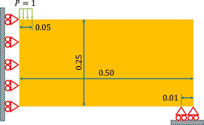
Elasticity problem: MBB beam
4.2 Results
The volume fraction is set to , and the MBB problem is solved by using all possible material models [i.e., combinations of interpolation domains (Sect. 3.1) and interpolation functions (Sect. 3.2)]. Generally, all models show typical behaviors where compliance drops dramatically during the first 25 iterations and gradually reduces until convergence. Similarly, the volumes fluctuate at the beginning, where many gray elements exist, but then stabilize until the iteration processes converge. For brevity, we only present the iteration histories using the triangular prism; see Fig. 16.
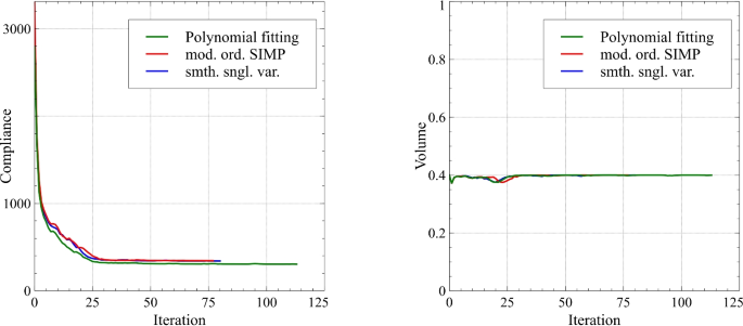
Iteration history when using the triangular prism domain
Figures 17, 18, and 19 show the optimized designs for all interpolation domains by using polynomial fitting, modified ordered SIMP method, and smooth single-variable interpolation, respectively. The optimized values of , , and are plotted in the upper, middle, and lower subplots, respectively.
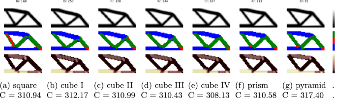
Optimized designs using polynomial fitting method and different interpolation domains. The optimized compliance values are given below the names of the interpolation domains
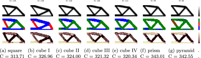
Optimized designs using Ordered SIMP method and different interpolation domains. The optimized compliance values are given below the names of the interpolation domains
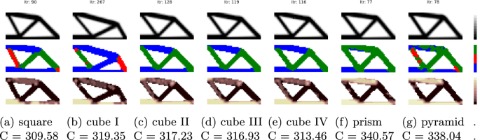
Optimized designs using the smooth single-variable interpolation method and different interpolation domains. The optimized compliance values are given below the names of the interpolation domains
Except in Figs. 18f–g and 19f–g, the designs have uniform distributions of lattices which also coincide with the directions of the principal stresses. For instance, the lower region of the design domain, where the shear stress is low, is filled with beige which corresponds to the square-shaped lattice (see Fig. 6) regardless of the color of . On the contrary, the shear stress is high in the middle of the design domain, making the -shaped lattice (red and dark brown ) more favored. At the left and right regions, where the vertical load and support exist, some material models have converged to the -shaped lattice (red and dark brown ) due to its dominant value, where the  -shaped lattice (blue and brown ) is occupying the upper region of the design domain where the normal stress (horizontal) is high.
Taking the optimized design of Fig. 17a as an example, we plot the corresponding two-scale structure in Fig. 20. As we see, the distribution of the lattices is uniform and the connectivity between the unit cells is generally good because our lattices have good connectives at the boundaries except the -shaped, and  -shaped lattices as they match only at the corners. However, when it comes to manufacturing the optimized structure, the small regions with doubtful conductivity might be slightly changed to their neighbor lattices, i.e., changing from 1 (lattice without outer frame) to 0.9 (lattice with a thin outer frame). This of course results in a small negligible compromise in compliance, as our demonstrated example shows almost zero reduction. Another possible solution is to include kinematical connectors as done in Hu et al. (2021) and Li et al. (2017).
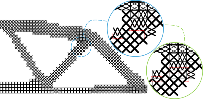
The corresponding microstructure for the optimized design seen in Fig. 17a. The blue zooming bubble shows some regions with doubtful connectivity surrounded by red dotted lines which has been manually modified (by changing from 1 to 0.9) as shown in the green zooming bubble. Compliance before and after the modification are 310.94 and 310.43, respectively. Further improved connectivity can be achieved by changing from 1 to 0.8, instead
Back to the lattices heterogeneity seen in Figs. 18f–g and 19f–g, the reason could be raised to the penalization () used in the modified ordered SIMP and smooth single-variable interpolations. In the following subsection, we study the effect of penalizing ψψ and in detail.