Article Content
1 Introduction
The generalized gamma (GG) distribution, which has many applications in different fields of science, is proposed by Stacy (1962). The probability density function (pdf) of the GG distribution is given as follows:
where and are shape parameters, is a scale parameter and stands for the gamma function. The GG distribution reduces to the gamma distribution and Weibull distribution for and , respectively. It also convergences to the log-normal and normal distributions as limiting cases. Besides, its hazard function can be monotonically increasing, decreasing, bathtub, or arc-shaped for different values of the parameters; see Cox et al. (2007) and Cooray and Ananda (2008). These properties of the GG distribution make it an attractive alternative for practitioners.
Although the GG distribution is mostly used for modeling purposes in the related literature, the maximum likelihood (ML) estimation of parameters of the GG distribution is problematic, as many authors indicate; see, e.g., Cooray and Ananda (2008) and references therein. The problem is because the corresponding likelihood equations include nonlinear function(s) of the unknown parameters, and thus, numerical methods should be utilized to solve them simultaneously. For example, Parr and Webster (1965), Harter (1967), and Hager and Bain (1970) are the first papers in which numerical methods such as Newton–Raphson (NR) used for this purpose. Later on, some researchers consider different estimation schemes. In this context, Prentice (1974) said that “existence of solutions to the log-likelihood equations is sometimes in doubt” and proposed an estimation method based on the re-parameterized log-density function of the GG distribution, namely log-GG, which is a member of the location-scale family along with a shape parameter . Then, Lawless (1980) stated that “…log-GG distributions with very different values can be similar, and this can create estimation problems …”; therefore, he presented the ML estimation for parameters of the log-GG distribution, when is assumed to be known. Recently, Noufaily and Jones (2013) rehabilitated the ML estimation—in a computational sense—by formulating a version of the likelihood equations of the GG distribution that two of them should be solved by numerically and the remaining one has an explicit solution. While the ML method has asymptotic desired properties, such as consistency, efficiency, and normality, it does not guarantee explicit form for the considered estimators. Therefore, numerical methods are usually employed to obtain the ML estimates. However, using numerical methods may cause various problems such as non-convergence of iterations, convergence to multiple roots, and convergence to wrong root; see, e.g., Puthenpura and Sinha (1986) and Vaughan (1992).
Based on the related literature, the authors believe that there exists considerable potential for improving the ML estimation of the parameters of the GG distribution. For example, obtaining an explicit solution for one of the likelihood equations of the GG distribution would dispel the doubt stated in Prentice (1974). Additionally, deriving the ML estimators of the location and scale parameters of the log-GG distribution explicitly, assuming the shape parameter is known, would contribute to the work of Lawless (1980). Furthermore, obtaining explicit solutions of two of the three likelihood equations would also contribute to the work of Noufaily and Jones (2013), where an explicit solution for one of the three likelihood equations was obtained. Therefore, in this study, we propose a new approach for estimating the ML estimates of the parameters of GG distribution by rehabilitating the approach given by Noufaily and Jones (2013) in some points by using the modified ML (MML) methodology, i.e., we obtain likelihood equations in which two of them have explicit solutions, and remaining one should be solved numerically. Since the MML method allows us to obtain explicit estimators, our approach contributes to previous approaches to solve the likelihood equations. In other words, the main contributions of this study are two-fold: (i) the solutions of two of the three likelihood equations are expressed in closed forms. Then, an interval containing the ML estimate of the shape parameter is provided. As a result, not only the result given by Noufaily and Jones (2013) has been advanced, but it also puts an end to the doubt mentioned in Prentice (1974). (ii) The closed-form estimators of the location and scale parameters of the log-GG distribution obtained in (i) are also robust. This result contributes to the study of Lawless (1980).
The rest of the paper is as follows. Section 2 is reserved for solutions of the likelihood equations. The proposed algorithm for parameter estimation of the GG distribution is presented in Sect. 3. The performance of the proposed algorithm is compared with the Broyden–Fletcher–Goldfarb–Shanno (BFGS) and Nelder–Mead (NM) methods in Sect. 4. The paper ends with some concluding remarks.
2 Solving the likelihood equations
Let X has the GG distribution with the pdf given in (1). Then, we consider variable-transformation and the following reparametrizations
where , , and are location, scale, and shape parameters, respectively.
The pdf given in (2) is the asymptotic distribution of the k-th extremes (k-th Extreme value distribution-EVk) proposed by Gumbel (1935) and also the particular case of the generalized Gumbel distribution introduced by Demirhan (2018). Note that the invariance property of ML estimation allows to obtain estimates of the parameters , and of the GG distribution as follows:
, , and .
2.1 The likelihood equations to be solved
The log-likelihood () function corresponding to the pdf given in (2) is
To simplify the mathematical operations, we use the following notation:
Then, the corresponding function is rewritten as
After differentiating the given in (3) concerning the parameters , , and k then setting them equal to 0, the following likelihood equations
and
are obtained. The likelihood equation given in (4) yields
which is an explicit expression for in terms of . However, likelihood equations given in (5) and (6) should be solved numerically, which may cause problems mentioned in the Introduction. It should also be noted that likelihood Eq. (6) allows us to obtain an interval including the estimated value of the shape parameter k. Equation (6) can be rewritten as
where is the digamma function. From the Theorem 1 of Alzer (1997), the right-hand-side of Eq. (7) is strictly monotonically decreasing (from down to 0), and since the left-hand side of Eq. (7) is greater than zero there must be a unique solution of the equation of interest, and thus the interval should contain as
2.2 The modified likelihood equations to be solved
Tiku (1967) proposed a methodology, which can be used for estimating the parameters of any distribution included by the location-scale family, to alleviate the mentioned computational difficulties in solving the likelihood equations for the location and scale parameters of a distribution. Since Tiku (1967), the MML methodology has been widely used for estimating the parameters of the different statistical distributions, see for example Kantar and Senoglu (2008), Akgul et al. (2016), and Arslan et al. (2021) in the context of Weibull, inverse Weibull, and Maxwell distributions, respectively. In recent years, the MML method has also been utilized to obtain solutions to various problems; see, for example, Alptekin et al. (2022), in which the MML approach was used to determine significant particle swarm optimization parameters.
2.2.1 The modified maximum likelihood estimation
In this subsection, explicit expressions for likelihood Eqs. (4) and (5) are obtained via the MML methodology. The steps of the MML methodology are given below.
- Step 1:Observations are ordered in ascending form, i.e., , and incorporated into the likelihood equations as
(9)
and
(10)where and .
- Step 2: function is linearized around the expected values of the standardized ordered observations, , by using the first two terms of Taylor series expansion:
(11)
where and denotes inverse of the upper incomplete gamma function.
- Step 3: function is replaced with its linearized form given in (11) in the Eqs. (9) and (10), then the modified likelihood equations
(12)
and
(13)are obtained. The modified likelihood Eqs. (12) and (13) yield explicit expressions
(14)for and in terms of k, where
Here, the denominator of the is replaced by for bias correction. See also Arslan et al. (2019) in which the MML estimators of the parameters and of the EVk distribution are already obtained.
Different than the previous approaches, here we do not need any numerical methods for solving the likelihood equations in (12) and (13) corresponding to the parameters and , respectively. In this context, problems encountered in numerical methods, e.g., non-convergence of iterations, convergence to multiple roots, and convergence to wrong roots, will be overcome.
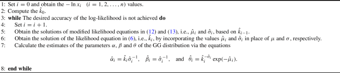
The remaining likelihood equation given in (6) can not be solved in closed form since it includes nonlinear functions of the parameter k; therefore, numerical methods, such as the NR, should be employed. The one-dimensional NR algorithm used for solving (6) has the following steps.
- 1:Set .
- 2:Give an initial value for the parameter , i.e., .
- 3:Obtain the value of by using the equation
- 4:If then stop else set and go to step (3).
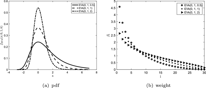
The pdf and weight plots of the EVk distribution,
Here,
where represents the trigamma function and and are the MML estimates of the parameters and , respectively, see Eq. (14).
Also note that bisection or Levenberg–Marquardt algorithms, which are available within the |MATLAB| function “fzero” and “fsolve”, respectively, can also be used for obtaining the solution of (6).
2.2.2 The properties of the modified maximum likelihood estimators
The MML estimators have remarkable properties, as shown below.
- The MML estimators of the parameters and are functions of the sample observation; therefore, they are expressed in closed form, remaining the same structure for any distribution.
- The likelihood Eqs. (4) and (5) are asymptotically equivalent to the modified likelihood Eqs. (12) and (13), respectively, i.e.,
see Vaughan and Tiku (2000). As a result, the MML estimators of the parameters and are asymptotically equivalent to their ML counterparts.
- The MML estimator of the parameter is expressed as the weighted mean of the sample observations, i.e.,
in which the small weight(s) are linked to the outlying observation(s) in the direction of the longer tail(s); therefore, it is robust to anomalies in the data. The pdf plots for different values of the shape parameter and the correspond weights () values are given in Fig. 1 for illustrative purposes.
- The MML estimators of the and are robust to plausible deviations from the actual value of the shape parameter; see, e.g., Acitas and Senoglu (2020).
2.2.3 Monte–Carlo simulation for the modified maximum likelihood estimators
The efficiencies of the MML estimators of the parameters and are shown via a Monte-Carlo simulation study. The simulations are conducted for runs where denotes the integer value function. Sample size, n, is considered as 30, 50, 100, and 500. The parameter k is taken to be 0.5, 1.0, 1.5, 2.0, 2.5, and 3.0, which were chosen arbitrarily, and simulations are performed in software |MATLAB2015b|. For each generated sample, the MML estimates of the parameters and are obtained; then, bias, variance, and MSE values of the MML estimators are calculated; see Table 1.
It can be seen from Table 1 that the simulated bias, variance, and MSE values of the and are reasonably small for the considered sample sizes. Also, the MML estimators are asymptotically unbiased, and the MSE values for the MML estimators of the parameters and decrease when the sample size increases, as the theory says.
The MML estimators can be obtained when the shape parameter k is known or a plausible value for the k has been assigned. However, it is known that the MML estimators of the and are robust to plausible deviations from the true value of the shape parameter k; see, e.g., Acitas and Senoglu (2020) and references given there. Therefore, we also investigated the corresponding robustness property of the MML estimators via a Monte–Carlo simulation under the different scenarios; see Table 2.
It can be seen from Table 2 that the MSE values of the MML estimators of the and are in acceptable limits even if the presumed value of the parameter k, say , is different than its actual value.
2.3 Plausible value for the shape parameter k
The MML estimators of the parameters and depend on the parameter k; therefore, a plausible value for the parameter k should be obtained. In this subsection, we use the method of moments (MoM) approach to obtain a plausible value for the k. As is well known, the MoM estimators are solutions to the equation system, which are obtained by equating the theoretical and sample moments. Here, we equate the expected value, variance, and skewness measures of EVk distribution with the sample mean, variance, and skewness, respectively. In other words, the following equation system should be solved to obtain the MoM estimates:
where
and is the th derivative of digamma function.
To obtain the MoM estimate of the shape parameter k, simultaneous solutions of Eqs. (16) and (17) are sufficient. Some simple algebra on (16) and (17) yields:
It is also known that
Then, the MoM estimate of the parameter k, say , is a solution of the following second-order differential equation, which is obtained by combining Eqs. (18), (19), and (20)
where , , and . Solution of differential equation in (21) can be obtained using the function |ODE45| available in |MATLAB2015b|. Here, is obtained via the similar steps in Demirhan (2018).
3 The proposed algorithm
The MML estimators of the parameter and have explicit forms which are functions of shape parameter k; see subsect. 2.2. Therefore, the parameter k should be known or estimated before obtaining solutions of the modified likelihood equations for and . Here, we use as a plausible estimate of k, say , in the initial step of the MML procedure; see Sect. 2.3. The proposed algorithm has the following steps.
The proposed algorithm
Also, the steps of the proposed algorithm can be shown in a flowchart as given in Fig. 2.
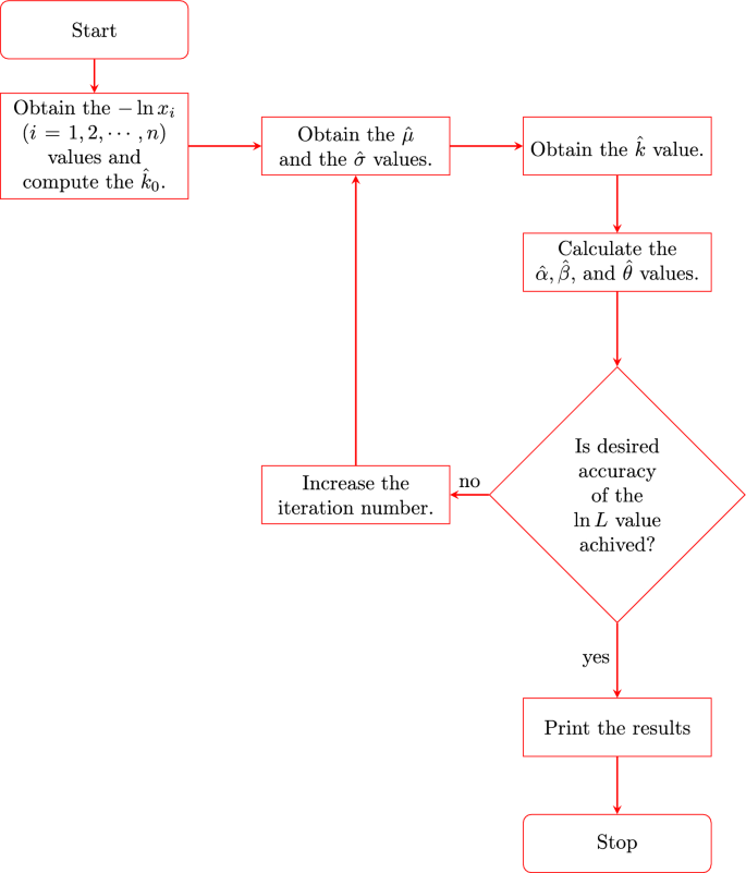
The flowchart for the proposed algorithm
We also conducted a Monte-Carlo simulation study to show the performance of the proposed algorithm. The simulations are performed for runs, and sample size, n, is considered as 100, 200, and 500. The different parameter settings chosen arbitrarily are considered, and simulations are performed in software |MATLAB2015b|. For each generated sample, the estimates of the parameters , and are obtained; then, the simulated bias, variance, and MSE values of , , and are calculated; see Table 3.
It can be seen from Table 3 that the proposed algorithm shows adequate performance in estimating the parameters , and of the GG distribution since the simulated bias, variance, and MSE values of the , and are in acceptable limits. Also, the simulated variance and MSE values of the , and obtained using the proposed algorithm decrease when the sample size increases, as expected.
4 Performance of competing algorithms
In this section, the GG distribution is considered for modeling two data sets in which one of them includes the survival times of 72 guinea pigs, and the remaining one contains the wind speeds data obtained from a meteorological station located at Sakarya in Türkiye. The estimates of the parameters of the GG distribution are obtained by using the proposed algorithm. Also, the well-known Broyden–Fletcher–Goldfarb–Shanno (BFGS) and Nelder–Mead (NM) optimization algorithms are utilized to compute the ML estimates of the parameters of the GG distribution. We refer to Ebadi et al. (2023) and references therein for the details of the BFGS algorithm.
4.1 Application-I
In this subsection, the GG distribution is considered for modeling the survival times data given in Table 4; see Bjerkedal (1960) for further information.
In analyzing the data, we first used the well-known BFGS and NM optimization algorithms for obtaining the ML estimates of the parameters of the GG distribution. The BFGS and NM algorithms are available within the |MATLAB| functions “fminunc” and “fminsearch”, respectively. We see that the BFGS and NM algorithms fail to give reliable results for different sets of initial values for the parameter , and , i.e., ; see e.g., Table 5. It is clear from Table 5 that the NM and BFGS algorithms converge to the wrong root when is (1.0, 0.5, 1.5). Also, their usage results in non-convergence of iterations and initial value problems; see Table 5.
We also extend the results given in Table 5 by using different sets of initial values to investigate how the initial value condition affects the NM algorithm. For this purpose, we generated a set of initial values consisting of 8000 triplets (, , and ); i.e., the initial value for each parameter is taken from the sequence having starting, end, and increment values 0.5, 10, and 0.5, respectively. The results show that the NM algorithm gives “-Inf” for 6960 initial values. We also get the following error message “Objective function is undefined at initial point. Fminunc cannot continue” in most of the cases. Since similar problems arise when BFGS is used, we do not report them here. Overall, the initial value may adversely affect the performance of the BFGS and NM algorithms.
On the other hand, we do not encounter any problems while using the proposed algorithm to estimate the parameters of the GG distribution. The proposed approach uses MML estimates, obtained explicitly and asymptotically equivalent to their ML counterparts. We calculated estimates of the , and of the GG distribution along with the corresponding value at each step of the proposed algorithm; see Table 6.
From Table 6, it is clear that the desired accuracy of the value is achieved at the 27th step with value − 390.8879, and the corresponding estimates of , and of the GG distribution are 6.9326, 0.2787, and 0.0008, respectively. After obtaining the ML estimates of the parameters of the GG distribution via the proposed algorithm, we used , and , given in Table 6, as an initial value for the BFGS and NM algorithms in estimating the ML estimates of the parameters of the GG distribution. Note that the values for the maximum number of function evaluations (MaxFunEvals) and maximum iteration number (MaxIter) were assigned to be 5000. Also, the number of iterations (NoIter) and CPU times for the proposed algorithm, BFGS, and NM algorithms are given in Table 7 for computational comparison purposes. The corresponding results are given in Table 7.
The results given in Table 7 show that the ML estimates obtained by using the BFGS and NM algorithms differ from each other when different initial values are considered. See also Table 5 in which the BFGS and NM algorithms fail to give reasonable estimates.
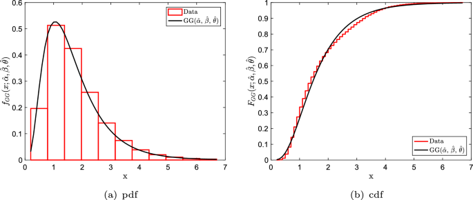
We also examine the goodness-of-fit of the GG distribution to the data by using Kolmogorov–Smirnov (KS) test. The KS statistics and its p-value are 0.10 and 0.42, respectively. Therefore, it can be concluded that the GG distribution fits the corresponding data adequately; see Fig. 3.
4.2 Application-II
In this subsection, the GG distribution is used to model the actual wind speed data, recorded hourly at 10 m height in 2009 from the meteorological station located at Sakarya in Türkiye. The sample size of the wind speed data set is 8750; see Arslan et al. (2017) for the details.
We obtained the estimates of the parameters , , and of the GG distribution by following similar lines in the previous subsection. The corresponding results are given in Table 8.
It is clear from Table 8 that the BFGS and NM algorithms give inconsistent results, similar to the previous subsection, based on the different initial values. Although the parameters of the GG distribution are defined on , the estimate of the parameter was obtained as − 0.0900 when the BFGS algorithm is used. Thus, it can be said that the BGFS algorithm could be adversely affected by the initial values and may fail to give a reasonable estimates of the parameters.
The results given in Table 8 show that the desired accuracy of the value, obtained via the proposed algorithm, is achieved at the 44th step with value − 10987.9171, and the corresponding estimates of , and of the GG distribution are 7.4795, 0.3844, and 6.7996e−04, respectively.
Arslan et al. (2017) used Weibull, power Lindley (PL), and generalized Lindley (GL) distributions, and the corresponding values of them are − 11493.4925, − 11601.9660, and − 11142.6418, respectively. However, the value of the GG distribution is higher than the Weibull, PL, and GL distributions; therefore, it can be concluded that the GG distribution better models the corresponding data than them. The fitting performance of the GG distribution is also illustrated in Fig. 4.
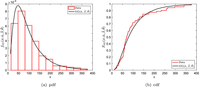
The pdf and cdf plots of the GG distribution with histogram and empirical cdf of the survival times data
The pdf and cdf plots of the GG distribution with histogram and empirical cdf of the wind speed data
5 Conclusion
The GG distribution is one of the popular distributions used in different areas of science. The reason why it draws the attention of practitioners is that it provides flexibility in terms of modeling and includes many well-known distributions as submodels. However, the ML estimation of the parameters of GG distribution is problematic.
In this study, we propose a new approach for estimating the ML estimates of the parameters of GG distribution by rehabilitating the approach given by Noufaily and Jones (2013) in some points. The parameters of the GG distribution are expressed as functions of parameters of EVk distribution, which is obtained by a transformation of GG distribution. Then, estimators of the location and scale parameters of EVk distribution are formulated explicitly. The estimates of , and k are used for calculating the estimates of the parameters of GG distribution. A simple algorithm, including the estimation steps, is also provided. Since the proposed approach depends on explicit estimators, no computational complexities or problems, such as non-convergence of iterations, convergence to multiple roots, and convergence to wrong roots, exist.
The proposed approach provides a guaranteed solution for the ML estimates of GG distribution, unlike the NM and BFGS algorithms. However, there is no guarantee that the resulting solution is the most efficient, i.e., we concentrate only on the computational task of maximizing the likelihood rather than on the inferential quality of the estimates. This question is also raised by Noufaily and Jones (2013) and should be considered in future studies. However, it can be concluded that the performances of the BFGS and NM algorithms could be improved when the estimates obtained via the proposed algorithm are used as initial values for them; see Tables 7 and 8.
Also note that although there are different estimation methods for estimating the parameters of a distribution, in this study, we focused only on the ML estimation of the parameters of the GG distribution. This is because some authors-referenced and discussed by Noufaily and Jones (2013)-have claimed that the ML estimation of the parameters of the GG distribution has computational complexities and certain deficiencies. Therefore, our primary aim in this study is to propose an alternative algorithm to solve the computational problems encountered in the ML estimation method used by many authors when estimating the parameters of the GG distribution rather than comparing the efficiencies of different parameter estimation methods with each other. However, the efficiencies of the estimators proposed in this study can be compared with those of other estimators existing in the literature. Additionally, it can be noted that the effects of alternative optimization techniques or algorithms on the computational efficiency of the proposed algorithm in the context of parameter can also be investigated.