Article Content
1 Introduction
A grillage is a planar network of intersecting beams, commonly employed to form bridge decks, building floorplates and other structures. Research on the optimization of elements forming building structures can be traced back to the 1950s and 1960s (Heyman 1959; Morley 1966), with work specifically on grillages carried out in the early 1970s; key research in this area was carried out by Rozvany and co-workers (Rozvany 1972a, b), and by Lowe and Melchers (1972, 1973). Although Rozvany’s original kinematic method provided a means of obtaining exact optimal grillage layouts for problems involving both single- and multiple-load cases (Rozvany 1972a), it could only be applied to clamped domains and required all loads to be orientated in a downward direction; it also did not furnish the optimal distribution of beam widths. While some of these restrictions were subsequently lifted (Rozvany et al. 1973; Rozvany and Hill 1976; Prager and Rozvany 1977; Rozvany and Liebermann 1994), and a computer program that allowed for automatic generation of analytical optimal layouts for arbitrary polygonal domains with partially clamped and simply supported boundaries was developed (Hill and Rozvany 1985), many restrictions still remained. For example, the cited analytical approaches could not be applied to problems involving free edges, interior simple supports, mixed downward/upward loadings, or point moment loadings. This severely affected the practical usefulness of the methods developed.
In all the aforementioned analytical investigations, the plastic design of grillages was considered in a continuous context, assuming a notional slab composed of an infinite number of fiber-like beams. An optimal fibrous slab can be compared with an in-plane Michell structure (Michell 1904), which often also includes fibrous regions, and is well known in the field of structural optimization (e.g., see Hemp 1973; Chan 1967; Lewinski et al. 1994a, b). A numerical means of identifying Michell-type structures was proposed by Dorn et al. (1964), and further developed by other workers (Gilbert and Tyas 2003; Sokól 2014; Zegard and Paulino 2014). To identify an optimal layout, a ‘ground structure’ comprising members interconnecting a grid of nodes distributed over the design domain was first created; optimization was then used to identify the subset of members present in the optimal (e.g., minimum volume) structure.
These numerical approaches stimulated Sigmund et al. (1993) and later Bołbotowski et al. (2018) to develop ‘ground structure’-based layout optimization approaches for grillages. However, only problems using coarse nodal grids were tackled by Sigmund et al. (1993); in developing a formulation that could be solved using linear programming (LP), and taking advantage of the computationally efficient adaptive solution technique proposed by Gilbert and Tyas (2003), Bołbotowski et al. (2018) were able to tackle problems involving many millions of potential beams. Their approach could also be applied to arbitrary design problems, free of the restrictions that had greatly limited the usefulness of earlier analytical approaches. In the plastic design formulation that was developed, the goal was to minimize the volume of material for specified applied loading, with the generated optimal layouts closely approximating the analytical solutions found by Rozvany et al. (1973) for a range of benchmark problems.
However, when using modern limit state design methods to design a structure, engineers need to consider not just the ultimate limit state (ULS), but also the serviceability limit state (SLS). This means that the plastic design considerations accounted for in the grillage layout optimization method described by Bołbotowski et al. (2018) should be coupled with elastic design considerations. To achieve this goal, a non-linear material model that includes both elastic and plastic regions must be considered. In analysis, non-linear material models are typically treated via iterative methods that utilize a tangent stiffness for each load step. An alternative method for determining the response of the non-linear model involves using an energy-based approach within an optimization framework. It is based on the principle of least action and often involves minimizing or limiting the strain energy (see, e.g., Stricklin and Haisler 1977; Ohkubo et al. 1987; Toklu 2004). Recent development has led to tools for energy optimization of reinforced concrete panels (Vestergaard et al. 2021, 2023a, b).
The energy method has been combined with material optimization. Kaliszky and Lógó (1997, 2002) optimized trusses in the framework of shakedown analysis. Klarbring and Strömberg (2013), Ramos and Paulino (2015) presented a method for hyper-elastic bodies using topology optimization. While Klarbring and Strömberg (2013) used two-dimensional elements, Ramos and Paulino (2015) used a truss-based ground-structure approach. Larsen et al. (2024) optimized reinforced concrete panels using Sequential Convex Programming consider multiple limit states.
In the present paper, the combined energy method and material optimization scheme for reinforced concrete panels tentatively proposed by Vestergaard (2022) (in a supplementary work chapter of his PhD thesis) is applied to beam grillages. And for the sake of simplicity, a truss representation of a grillage is adopted. The novelty of the approach lies in the incorporation of displacement and strain constraints on the grillage, while accommodating both elastic and elastoplastic material behavior. In addition, multiple-load cases are incorporated, allowing for more realistic loading scenarios that account for both SLS and ULS criteria, while still ensuring minimal material usage.
The paper is organized as follows: in Sect. 2, a truss optimization formulation capable of handling non-linear material models and displacement and strain constraints is described and then used as the basis of a grillage optimization formulation; in Sect. 3, the approach is applied to a range of examples, from simple benchmarks to more geometrically complex problems, including a building floorplate comprising 16 supporting columns; these results are discussed in Sect. 4 and the conclusions drawn in Sect. 5.
2 Formulations
2.1 Truss optimization
Here, the optimal grillage problem is, for the sake of simplicity, formulated using a truss model. In the model, three-dimensional bar elements are used; each element has a cross-sectional area, , and a constant normal force, , where e is the element number. In this case, the element is a stress-based (force-based) element, where the degree of freedom (DOF) in the element is the normal force rather than the displacement.
The material is characterized by its Young’s modulus, E, and the yield stress, , at which point perfectly plastic behavior follows, as illustrated in Fig. 1.
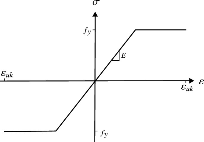
Linear elastic-perfectly plastic behavior ( = ultimate strain)
The response of a structure can be found by utilizing the principle of minimum complementary energy, which states that of all stress fields in an elastic body that satisfy equilibrium and stress boundary conditions, the one that also satisfies compatibility will minimize the complementary energy. The material model given in Fig. 1 can be approximated as a hyper-elastic model, and since only monotonically increasing loads are considered, the behavior of an elastoplastic and hyper-elastic model is identical.
For a truss structure with this material behavior, the complementary strain energy, , is given by
Here, is the normal stress, is the element length, is the domain of the structure, and is the number of elements.
Equilibrium is expressed by stating that the sum of internal forces at a given node should equal the applied load at that node. This can be achieved using an equilibrium matrix, , given as
where is the unit direction vector of the element, and is the system DOF numbering of the element. and are the element-wise equilibrium matrices on element and system levels, respectively. Thus, equilibrium can be written as
where is a vector of all normal forces and is the load vector.
Yielding of the bar elements can be implemented by limiting the normal force in the elements to the yield force. This can be written as
This can be stated in matrix form for all elements as
where is a vector containing the areas of all elements.
To produce optimized structures, the principle of minimum complementary energy is combined with material optimization, such that the volume of the structure is minimized. This can be stated as a weighted sum of the complementary energy and the material usage, which is a multi-criterion optimization problem
where is a vector containing the lengths of all elements, is the weighting on the potential energy of load case i, is the weighting on the volume, and is the number of load cases. Equation (6) is a Second-Order Cone Programming problem, which can be solved efficiently via modern solvers, e.g., Mosek ApS (2023). Furthermore, as the objective is convex, all solutions can be found using the linear scalarization approach. From the above optimization problem, the dual problem can be derived (for derivation, see Appendix)
In the dual problem, and are vectors containing the total and plastic strains for load case i, respectively. is element e of . is the displacement vector of load case i, while is the displacement vector of element e with respect to load case i. is the strain interpolation matrix. Note that the inequality in the equation must hold for all elements on the right-hand side. Thus, the objective of the dual problem is to minimize the potential energy; from this, the dual variables (i.e., the displacements and the strains) can be obtained.
As seen from the dual problem, the value of can be chosen as a limit on the strains or displacements of a given load case. Thus, an iterative method can be formulated in which the value of is chosen as unity; subsequently, Eq. (6) is solved. Hereafter, the strains or displacements are compared to a given limit. If the limit is exceeded for load case i, the value is increased corresponding to the utilization. The same is true of the strains that are below the limit, where the value of is decreased. This is illustrated in Algorithm 1.
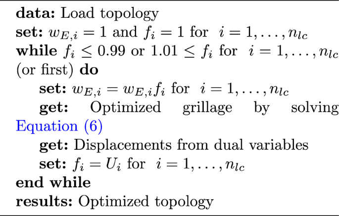
Optimization scheme
where or for restrictions on strains or displacements, respectively.
This heuristic approach solves the problem efficiently, with simple cases using less than five iterations and up to ten iterations for more complex examples. For single-load cases, the termination of the iterative process is guaranteed, which is also true for most practical examples with multiple-load cases. Designed examples with identical load cases but different load levels do not terminate. However, this is not deemed a problem, as the non-governing load case can be removed from the optimization.
2.2 Grillage optimization (truss formulation)
The truss optimization formulation will now be used to find the optimal layout of beams forming a grillage subjected to out-of-plane loading. A layered model is used, with the two layers representing the top and bottom parts (e.g., ‘flanges’) of a typical beam member. To compare the results with current methods, the areas of the top and bottom flanges are chosen to be identical. Furthermore, to correctly carry shear, a mesh connecting the top and bottom layer, representing the web, must be included. The web elements are excluded from the volume in the objective function, such that the area can be chosen freely with no penalty. The flanges are thus the only contributor to the volume part of the objective function. The ground structure is shown in Fig. 2.
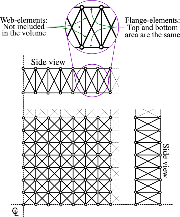
Illustration of ground-structure mesh (assuming adjacent connectivity)
The support conditions must be modeled to describe the supports accurately. Three different kinds of supports are used in the present study, which are shown in Fig. 3.
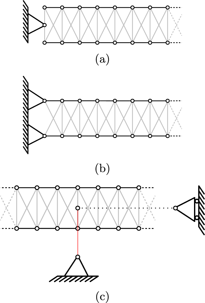
Truss model representation of the different support types, with gray elements being web elements (free area): a simply supported boundary (only supporting vertical load); b fixed supported boundary; c internal column support, with the red line indicating the column that connects to a node positioned at mid-depth and the dotted black line indicating the support placed at the mid-depth node
For support (a) and (c), additional constraints are added to ensure against rigid body motion.
2.3 Single beam example
To investigate the truss formulation, a pin-supported beam is studied. Two load cases are considered (Table 1), one at the quarter span and the other at the three-quarter span, as shown in Fig. 4.
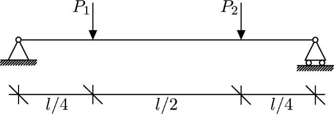
Single beam example: problem definition
An analytical expression for the optimal layout for Load Case 1 (LC1) can be calculated as
where is the moment for LC1. For two load cases, the optimal layout can be determined as follows:
where is the moment for Load Case 2 (LC2) given by
The optimized beam for the structure loaded by both LC1 and LC2 is shown in Fig. 5, where the size of the flanges is shown alongside the displacements of the two load cases.
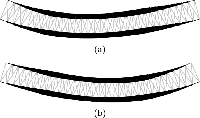
Displacements of the truss model of the single beam test subjected to both load cases: a load case 1; b load case 2 (Gray lines indicate the ‘free’ web elements.)
Figure 5 illustrates the truss representation of the beam, the optimized area of flanges, and the displacements. However, for thin plates with a large thickness-to-length ratio, this representation becomes unsuitable. Since the area of the top and bottom layers is identical, only one layer is shown for the following examples, with colors indicating hogging moments (red) and sagging moments (blue). For displacement plots, the average displacement of the corresponding top and bottom nodes is used.
Figure 6 compares the flanges of the beams in both analytical and numerical solutions. The optimized beam for two load cases has a volume of when allowing for fully plastic actions, coinciding with the analytical solution. However, contrary to what is expected, when limiting the strains to the yield strain, , through the iterative process described in Algorithm 1, the value becomes . This is due to the interaction between the limit on the strains and the weighting on the complementary energy. When the weighting increases, the corresponding relative weight on the volume decreases. When the limit on strains becomes high, and the weighting approaches infinity, the weight on the volume relatively approaches zero. Hence, the algorithm can find a better overall objective value by increasing the volume and thus decreasing the complementary energy. Therefore, the method can find optimal solutions for low-strain constraints (fully allowing plastic deformations). However, only close to optimal solutions are found when using strict strain requirements.
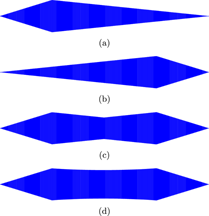
Single beam test: a optimized beam for LC1; b optimized beam for LC2; c optimized beam for LC1+LC2 (); d optimized beam for LC1+LC2 ()
This behavior is, however, not seen for a single-load case; this is thought to be due to the total complimentary energy for two load cases being much larger than for one, resulting in different weightings. The behavior is shown in Fig. 7.
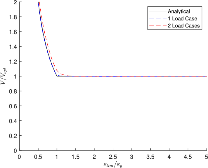
Single beam test: evolution of volume for different strain requirements
As seen in Fig. 7, the error is, in general, small, with the highest error found when , at 7.6%. When considering multiple-load cases, compatibility is still guaranteed, as the complementary energy for a chosen layout is independent. Thus, the complementary energy of all load cases will be at a minimum for the given layout, ensuring compatibility. However, the material consumption is not necessarily at a global minimum, as shown in the analysis.
The convergence with respect to the number of elements is also investigated when . The convergence behavior is shown in Fig. 8.
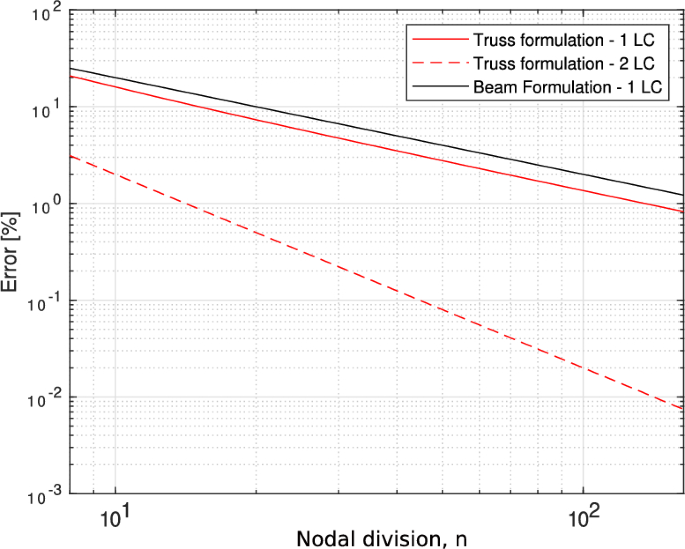
Single beam test: convergence compared to beam formulation given by Bołbotowski et al. (2018) (percentage error calculated using the analytical solution)
The figure clearly shows that the solutions from all methods converge toward the analytical solution for increasing nodal division. Furthermore, convergence is slightly faster than the traditional beam formulation in the test with one load case, which is likely because the truss formulation permits different normal forces in the top and bottom layers and, consequently, more freedom in the design.
3 Examples
To ensure well-scaled problems, a scaling factor is used on the forces and lengths in the following examples. For all examples, the forces in Newton are scaled by a factor of , and the lengths in meters are scaled by . These values are chosen empirically and proved to perform well for all examples. Furthermore, for the sake of simplicity, all loads are applied evenly between the top and bottom layers.
3.1 Uniformly loaded square domain problems
Two simple benchmark examples are used to validate the method described against available analytical and numerical solutions. Both examples involve square domains and uniform out-of-plane loading; the first has simply supported boundary edges, and the second has fixed corner supports, as illustrated, respectively, in Figs. 9a and 10a. Blue and red lines indicate sagging and hogging beams, respectively:
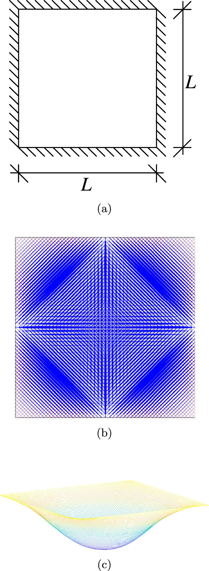
Uniformly loaded simply supported square domain problem: a problem definition; b optimized grillage; c displacements for a simply supported problem
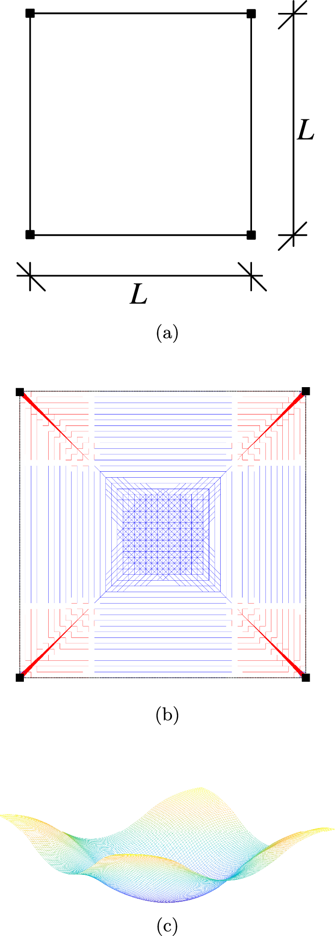
Uniformly loaded fixed corner square domain problem: a problem definition; b optimized grillage; c displacements for a fixed corner supports problem
The optimal grillages are presented in Figs. 9b and 10b, solved using a nodal division of per side. The results are very similar to the analytical solutions presented by Morley (1966) and Rozvany (1972b), respectively. When using a higher nodal division of , the optimal volumes reported by the method are and (where ), which are also very close to the analytical solutions ( and , respectively). The differences are thought to be due to the constant truss element used, compared to an element with a linear cross-sectional area variation. To further investigate the solution, the displacements from the dual variables are presented in Figs. 9c and 10c. The displacements are as expected, with the largest displacement in the center of the domains. A convergence plot for the two solutions is given in Fig. 11, where it is compared to the standard beam formulation given by, e.g., Bołbotowski et al. (2018). Note that in the beam formulation, beams are kept non-tapered to more accurately represent the truss mesh shown in Fig. 2.
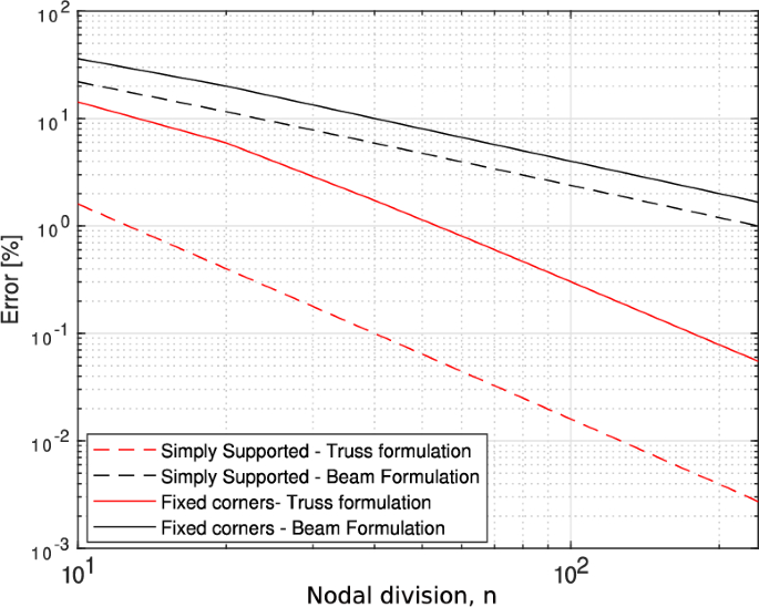
Uniformly loaded square domain problems: convergence characteristics
The relative error for both examples is seen to approach zero in both cases, indicating that the method does converge toward the optimal solution. For both examples, the truss formulation converges faster than the beam formulation due to the same effect explained previously in Sect. 2.3.
3.2 Domain with internal line supports
In addition to the benchmark examples, more complex examples are also investigated. The first structural example is a square domain with internal line supports, as shown in Fig. 12.
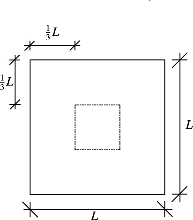
Domain with internal line supports: problem specification
Three load cases are considered; see Fig. 13.
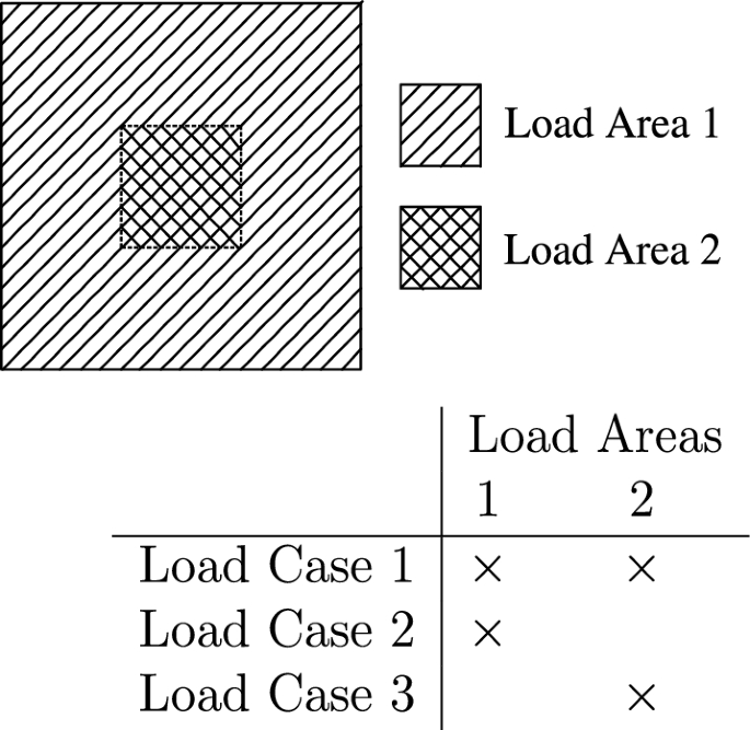
Domain with internal line supports: illustration of the load areas and load cases
The resulting grillage is shown in Fig. 14a, and the optimal volume is . Figure 14b–d illustrates the displacements for each load case.
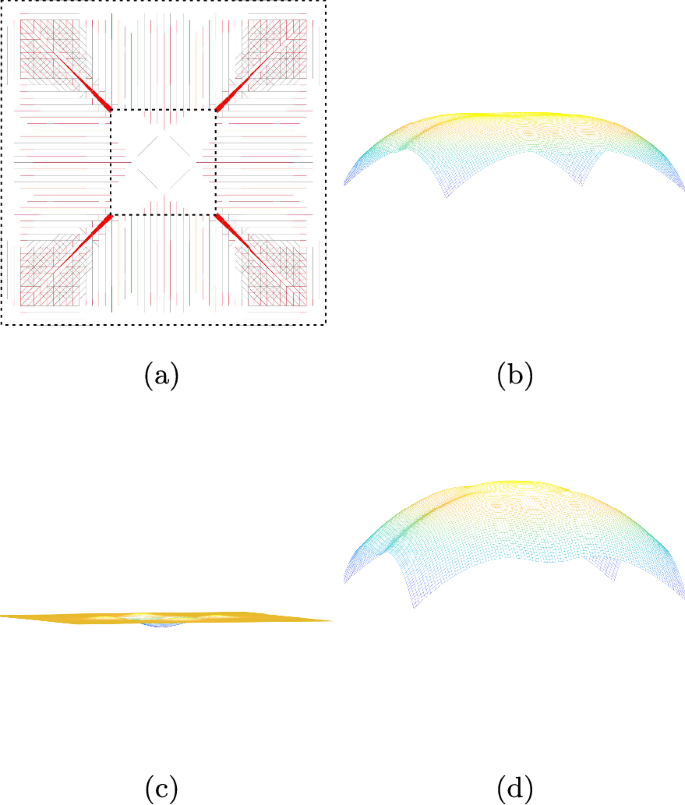
Domain with internal line supports: a optimized grillage layout plotted for ; b displacement under Load Case 1; c displacement under Load Case 2; d displacement under Load Case 3
The optimized grillage in Fig. 14 shows that the method can handle multiple-load cases, and that the structural responses of all load cases can be identified. For the examples with multiple-load cases, the color indicates a combined behavior for all load cases. Red indicates hogging in all load cases, blue indicates sagging in all load cases, and gray indicates a mixture of hogging and sagging. The transverse displacements are the largest for Load Case 3.
3.3 Domain with L-shaped hole
The next example is a square domain with an L-shaped hole, which has a mixture of fixed and free boundaries; see Fig. 15.
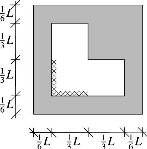
Domain with L-shaped hole: illustration of a domain with an L-shaped hole and both free and supported edges
Three cases are considered: one with a point load in the inner corner, one with a point load in the upper right-most corner, and one with a distributed load. The optimized layout for all three cases is given in Fig. 16, with an optimal volume of , , and , for cases 1, 2, and 3, respectively.
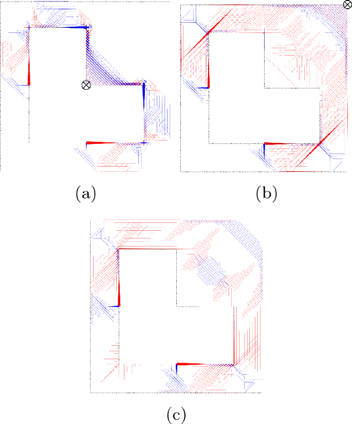
Domain with L-shaped hole: optimized grillage solutions for three different loads, plotted for : a Case 1—point load in the inner corner indicated by ; b Case 2—point load in the upper right-most corner indicated by ; c Case 3—uniformly distributed pressure load
The solutions are not identical to those found by Bołbotowski et al. (2018), though the layouts remain somewhat similar. This is due to the difference in ground structures: here, only members oriented at 0°, 45°, and 90° are present in the ground structure, whereas Bołbotowski et al. (2018) utilize full connectivity. As a result, the optimal volume reported here is 15–30% above that found by Bołbotowski et al. (2018). If the same ground structure is employed, the difference in volume between the two approaches is within 2%.
In Fig. 16b, a pattern of orthogonally intersecting hogging and sagging beams can be observed along the edges near the point load. This is the so-called ‘beam-weave’ phenomenon, also discussed by Rozvany and Liebermann (1994) and Bołbotowski et al. (2018).
Since multiple-load cases are essential in civil engineering, the following study considers three load cases. To ensure that the optimal design is not dominated by a single-load case, the point loads are defined as for load case 1 and for load case 2, while the uniformly distributed load in load case 3 is given by p.
First, the three load cases are considered separately, so the outcome layout is an overlap of the three designs in Fig. 16. And the member area is the maximum cross-sectional area among all load cases
where is the area of bar e, while , and are the areas for bar e for the optimal layout of load cases 1, 2, and 3, respectively. This leads to an estimate of the total volume given as .
Second, all three load cases are considered simultaneously. The optimized layout is shown in Fig. 17a and the total volume is , revealing a saving of 22.4% compared to the case where the load cases are considered separately.
To further show the potential of the proposed method, different material behaviors and limits are considered. In Fig. 17a, b, limits on the strains of and are applied, respectively. Figure 17c imposes a limit of L/100 on the transverse displacement. It can be observed that different material behaviors result in different resulting layouts. Also note that different material behaviors can be assigned to different load cases for more realistic designs. For example, some load cases can be associated with linear elastic material behavior, while others can allow for elastoplastic behavior.