Article Content
1 Introduction
CAD-free, parameter-free, grid-based, or node-based shape parameterizations have matured into a potent tool in structural optimization. Besides Eulerian shape formulations like level-set methods (Allaire et al. 2004) or density-based methods (Bartz et al. 2021), the success of these Lagrangian descriptions has also been recognized in the industry. Unlike CAD-based methods or similar techniques, node-based optimization changes the shape by relocating every FEM grid node individually. This leads to the largest achievable design space and thus requires adjoint sensitivity analysis to compute gradient information efficiently and proper regularization techniques, which in shape and topology optimization are called filtering or smoothing methods.
Filtering can generally be categorized into two types: explicit or implicit. The implicit approach generates smooth designs by solving an elliptic PDE. Various implicit filters have been proposed in the literature by choosing a different underlying equation. The traction method, also known as gradient method of Azegami and Wu (1996), intuitively selects the elasticity problem, well known by structural engineers. Jameson and Vassberg (2000) introduced gradient smoothing using the Sobolev filter. Lazarov and Sigmund (2011) successfully applied implicit filtering in topology optimization. An extraordinary overview of implicit filtering is given in Swartz et al. (2023), and Radtke et al. (2023) has conducted an excellent, in-depth mathematical analysis of explicit and implicit filtering. Parallel to the development of implicit filtering, the smoothing of fields by convolution of kernel functions, known as explicit filtering, has been studied. Starting from treating the checkerboard problem in density-based topology optimization (Sigmund 1994), it found its way into shape optimization problems (Le et al. 2011).
Bletzinger (2014) and Hojjat et al. (2014) demonstrated how explicit filtering is implemented into a consistent frame by introducing the Vertex Morphing method, a shape parameterization technique designed for first-order gradient-based optimization. The Vertex Morphing method succeeded in optimization problems of industrial importance (Hojjat et al. 2014; Najian Asl et al. 2017) and was continuously explored. Algorithms for constrained optimization, especially suitable for the Vertex Morphing method, have been established by Chen et al. (2019) and Antonau et al. (2021). Geiser et al. (2024) removed discretization dependencies and improved the convergence behavior by applying a consistent variable scaling scheme based on the shape morphing function. Najian Asl and Bletzinger (2023) introduced implicit filtering based on the Laplace-Beltrami operator into the Vertex Morphing framework for optimizing bulk-surfaces and studied the differences to explicit filtering. Recently, Meßmer et al. (2024) presented a combination of this implicit Vertex Morphing with embedded boundary methods to optimize the shape of solid structures, decoupling the geometry description from the finite element discretization to eliminate mesh distortion problems.
Although there exists an immensely rich source of material in the research fields of sizing, topology, and shape optimization separately, a combination of these techniques has been rarely examined, even less in a simultaneous manner, in which the design variables are collected into a single vector and given to the optimization algorithm as one complete set. Maute and Ramm (1997) investigated combined shell shape and topology optimization in an alternating approach, in which the design mesh could also be adapted through the optimization. Staggered shape and topology optimization procedures have also been proposed by Christiansen et al. (2015); Riehl and Steinmann (2015), and Lian et al. (2017). Arnout et al. (2012) optimized the thickness of previously shape-optimized shell structures using explicit sensitivity filtering. Zhou et al. (2004) conducted early work on the simultaneous treatment of different design variable types, focusing on bead design with small shape changes. Hassani et al. (2013) parametrized the shell midsurface using NURBS and employed Solid Isotropic Material with Penalization (SIMP) for the concurrent topology optimization. NURBS-based descriptions for density-based topology, thickness, and material anisotropy have further been successfully formulated to solve simultaneous optimization problems of continua, see Costa et al. (2019), Montemurro (2022); Montemurro and Roiné (2024), and Montemurro et al. (2024). Herein, the local support property of NURBS automatically avoids mesh dependency and the checkerboard effect. Furthermore, the minimum length scale requirement is effectively addressed by tuning the parameters of the NURBS basis functions without introducing an explicit constraint in the problem formulation. One of the first studies using parameter-free shape optimization unified with density-based topology optimization to increase the design space was presented by Shimoda et al. (2021), in which a Poisson’s equation (heat conduction problem) for smoothing the scalar density design variables was added to the traction method. Another parameter-free shape parameterization concurrently combined with SIMP was recently proposed by Kamper and Naets (2024). There, explicit filtering for narrowly bounded shape variables is applied. Despite this limited design space, the simultaneous method shows potential as it can yield better results than sequential schemes.
Papoutsis (2023) and Träff (2023) have submitted the thematically closest works to this paper. Papoutsis (2023) extended the explicit Vertex Morphing method with scalar variables for topology optimization. Inspired by SIMP, a Sigmoid function incentivizes the scalar variables to reach a black-white design. Additionally, a root-finding problem is solved in each optimization iteration to enforce an update of shape and topology variables by a predefined and fixed step size for each individual. This strategy was strongly driven by industrial application, where adequate designs must be found in a reasonable time in highly constrained optimization problems. Träff (2023) proposed a simultaneous shell shape and thickness optimization methodology that utilizes implicit Laplace–Beltrami filtering based on the initial geometry configuration for both design variable types. The optimization problem of minimizing the strain energy while obeying a certain volume fraction, typical in topology optimization, is appended by a finite element metric constraint to improve the mesh quality through shape deformations. The problem was solved using the Method of Moving Asymptotes (MMA).
1.1 Contribution
In this work, shape and sizing optimization of thin-walled structures are unified in a fully concurrent optimization algorithm receiving both design variable types in one complete vector. The concurrent optimization problem is formulated in Sect. 2, not including any additional mesh quality constraints because it is unnecessary as Vertex Morphing controls mesh quality on the fly, leading to a simple but efficient formulation.
To solve the optimization problem, we work out the following steps:
- The explicit Vertex Morphing method for parametrizing the shape is revisited in Sect. 2.1, and a modification of Vertex Morphing is developed to control the shell thickness distribution in a parameter-free way in Sect. 2.2. The reformulation evaluates the explicit filter kernel on the initial mesh configuration and is invariant to shape changes. It is specifically designed to fulfill the thickness limits.
- The Relaxed Gradient Projection algorithm is adjusted in Sect. 2.3 to include variable bound constraints by adding a projection method. The modifications ensure that the thickness bounds are never violated throughout the optimization. A shell thickness optimization example demonstrates the performance of this strategy (Sect. 2.3.1).
- A variable scaling strategy is introduced to deal with the two variable types for concurrent optimization. The two design variable types are scaled concerning their physical dimension without using second-order information to make a simultaneous optimization possible (Sect. 3.1). The positive effect on the convergence behavior is shown in Sect. 3.1.1.
- The discretization-independent variable scaling approach for the Vertex Morphing method (Geiser et al. 2024) is revised in Sect. 3.2 for the explicit filtering on the initial geometry. The removal of the discretization dependency is briefly examined in Sect. 3.2.1.
The proposed concurrent method is tested in Sect. 4 on examples from the literature to create comparability. Finally, the approach’s applicability to an optimization problem of industrial importance is critically studied.
2 Vertex Morphing
Consider the constrained shape and thickness optimization of a thin-walled structure in a combined manner as
where J is the objective function, field describes the midsurface, t is the thickness field, and are inequality and equality constraint functions, and the last equation shows linear bound constraints on the thickness. While unconstrained optimization problems are viable for shape design variables, for example, minimizing just the strain energy, thickness variables usually require constrained optimization problems. Otherwise, trivial solutions would be acquired; for instance, strain energy minimization leads to an indefinite thickness increase, or unconstrained mass minimization results in a zero field.
This section first reviews the Vertex Morphing method as a parameterization technique to control the shape of the shell midsurface, and then, based on this explicit filtering scheme, an extension to control the shell thickness is carried out.
2.1 Shape filtering
The explicit filtering operation of the Vertex Morphing method generates a smooth shape from an introduced design control field through a convolution integral on the current geometry configuration with convective surface coordinates :
where is the surface coordinate of point i with spatial coordinates , and is the filter function, also called filter kernel. The choice of the filter function affects the obtained shapes and their geometrical properties. Linear functions are popularly used, as they already generate cubic surfaces for a linear discretization of the control field. They are defined as
Furthermore, Gaussian kernel functions are frequently utilized,
which yields a first-order approximation of Sobolev-based implicit filtering, see Stück and Rung (2011). Figure 1 shows the generation of a smooth curve by the filter procedure in 2D.
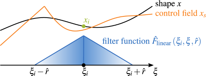
Shape filtering in 2D
The filter function is rewritten in a simplified notation, as in Antonau et al. (2022) and Najian Asl and Bletzinger (2023),
by using the spatial and not the surface coordinates to evaluate the filter function:
whereby a back relation between the left and the right side appears, which is commented on later. We notice that the filter functions and , and the radii and r are not the same. Even though they define the same linear function in their respective space, they differ if we would express them in the other space.
Equation (6) is usually discretized by standard finite elements. In application, the grid of the numerical analysis for the underlying physical problem is directly chosen to discretize the geometry of the shape optimization as well, minimizing the effort to set up the optimization problem. This leads to the approximations for the shape and the discrete design control field , which, inserted in the continuous form, results in:
or in abbreviated notation:
where is the jth entry of the ith row of matrix , known as mapping, filter, or morphing matrix, which reflects the filter effect as a linear interaction between control field and geometry:
The columns of the morphing matrix are called morphing functions. One can observe that node is obtained by a weighted sum of the control field in the vicinity, so the operation is dependent on the number of neighboring control field values. As a consequence, the consistency property is violated, which postulates that a constant control field develops a constant geometry (Najian Asl et al. 2017). To overcome this flaw, each filter function is scaled such that:
holds. This is often realized in the discrete form by normalizing the rows of the filter matrix by the -norm:
An approximation of the filtering operation is adequate in practice, and a midpoint Riemann sum numerical integration can be applied (Baumgärtner 2020), for which the filter function is evaluated at the control field nodes and multiplied by the nodal area, or rather, the diagonal (lumped) control field mesh matrix .
The aforementioned shape filtering technique is specially designed for first-order optimization methods, for which the control field is chosen as the design variable. In other words, the initial shape optimization problem is transformed from the physical design surface to the introduced design control field . The chain rule of differentiation is used to convert the gradients of a response function J:
This is known as sensitivity filtering or backward filtering, contrary to shape filtering or forward filtering, as shown in (9). Optimization is carried out in the design control space after the gradients of the objective and constraints function have been mapped to it.
For unconstrained problems, the steepest descent method has been successfully applied with explicit filtering, e.g., in Bletzinger (2014) and Firl et al. (2013). The design control update reads as follows:
where is a chosen step size, and the physical shape update is generated via the forward filtering:
The Vertex Morphing method can be interpreted as transforming the original optimization problem from the physical design space to the design control space . Hojjat et al. (2014) and Bletzinger (2014) presented that the optimization problem is not modified by explicit filtering and global and local minima are not changed. Node-based shape optimization of thin-walled structures, especially shells, is characterized by a non-convexity with many local minima. A large number of design variables is not the only reason for this non-convexity; it is also due to problem’s physical properties in the discrete and continuous setting. Firstly, the discretized problem features numerical issues, such as creating undesired element distortion, which creates artificial stiffness due to an ill-conditioned Jacobian or locking phenomenon. Secondly, the continuous problem is non-convex. For example, stiffness maximization of a flat plate loaded vertically possesses many local optima depicted through variations of local stiffeners (beads, regions of high curvature) and one global optimum of a shell with lower curvature shaped like a minimal surface. Which of these optima is found ultimately depends on the optimization algorithm. As a consequence of these challenges, engineers are generally satisfied to obtain a design at a local optimum. The Vertex Morphing method steers the non-convex shape optimization problem to a smooth shape in the direction of an optimum. Larger radii yield optimal shapes with smaller curvature and less waviness. Design features smaller than the filter radius are preserved, which is advantageous for industrial applications. The filter radius acts as a design handle, allowing the engineer to choose an optimal design. However, to regularize the shape optimization problem properly, a minimum filter radius of 4 times the element length is recommended.
Alongside their non-convex nature, node-based shape optimization problems are complex to solve with numerical optimization techniques due to several other aspects. A large number of design variables has to be managed, often reaching several millions. Objectives and constraint functions are mostly non-linear. Adjoint methods are preferred to obtain response sensitivities. Sensitivity analysis is not always analytically solvable, and semi-analytic sensitivity analysis is employed to partially approximate gradients. Additionally, the computation of response function values and sensitivities is numerically expensive. It usually takes up to 80% of computation time in one optimization iteration. Line search techniques are consequently numerically expensive, requiring more function evaluations or sensitivity computations. Furthermore, line search algorithms are not guaranteed to be beneficial for non-convex optimization problems with a starting design far from a target. They mostly exchange no more than the reachable local minima despite the additional numerical effort. Only close to a local optimum may they eventually secure the convergence if necessary. However, the overall quality of the optimization result does not significantly change due to this. Second-order optimization methods, such as sequential quadratic programming (SQP), require second-order information, which is usually not available and would be costly to compute for a large number of design variables. Line search techniques would generally be necessary when using Quasi-Newton Hessian approximations instead. Aside from that, the explicit filtering operation is eliminated by Newton methods (Bletzinger 2014). This can be shown by inserting the forward and backward filtering operations into the Newton update rule of the design control variables:
The aforementioned characteristics are the basis for the rationale to solve constrained Vertex Morphing-based optimization problems using first-order algorithms, which require a low amount of response function value and sensitivity computation. Chen et al. (2019) proposed a modified search direction method of the interior-point algorithm class. It applies a singular-value decomposition for the normalized response gradients to obtain a search path that traverses inside the feasible domain toward a local minimum. Another successful algorithm based on Rosen’s gradient projection (Rosen 1961) has been developed by Antonau et al. (2021): the relaxed gradient projection method. It mitigates the zigzagging behavior of active-set methods by activating the constraints before leaving the feasible domain. Line search techniques are mostly avoided, and a fixed step size is used for industrial applications.
It has to be stressed that the filter computation on the current geometry in Eq. (6) is indeed a recurrent relation, as the filter function (right-hand side) depends on the current geometry (left-hand side). Previous publications ignored this non-linearity, besides Najian Asl (2019), who indicates that this effect is negligible in the regime of small shape changes. Nevertheless, the filtering computation on the current geometry possesses a beneficial property: self-penetration of the design surface is virtually omitted during the optimization. Another aspect of the Vertex Morphing framework is that the design control field is typically unknown during the whole optimization process. It could be determined if one finds the dual filter, the inverse operation of the filtering (Bletzinger 2014), but this is unnecessary. Equation (14) shows that the shape change can be derived just by the update of the design control field.
Due to these characteristics, applying linear bound constraints directly on the design control variables becomes challenging and is formulated concerning the shape variables themselves, causing a non-linear constraint because of the filter operation linking the two variables, see Antonau (2023). As it is, generally more challenging for optimization algorithms to stay inside the feasible domain for non-linear constraints, it cannot be guaranteed that the variables are kept between the minimum and maximum values. Especially in the context of thickness optimization, it is crucial to satisfy variable bounds to prevent physically meaningless results like negative shell thickness values. It motivates to reformulate the Vertex Morphing filtering frame regarding the thickness variables in the following.
2.2 Thickness filtering
We aim to modify the Vertex Morphing method for thickness variables The modified filtering does not alter with shape changes It enables to determine the design control field so that linear variable bounds can be imposed directly on the design control field. Inspired by Träff (2023), the point of view concerning the design variables is slightly shifted. The current design thickness t at any point during the optimization is determined by:
where T is the initial thickness field of the initial configuration, and is the total thickness change, not to be mistaken for the shape update of one optimization iteration in Eq. (14). Sensitivity analysis is conducted on a physical model using the current design thickness, and hence, objective and constraint gradients are obtained with respect to the current design thickness. The chain rule is applied to convert them with respect to the total thickness change:
The convolution filter integral can now be employed on the initial configuration of the midsurface geometry:
where is the total thickness change field sampled at , which is the position vector of the geometry in its initial configuration, and is the design control thickness field. We propose the filter operation on the initial configuration to be called as initial filtering, in contrary to the established Vertex Morphing filtering for shape variables acting on the current configuration as updated filtering.
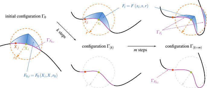
Filter function (left) formulated on the initial configuration and filter function (top) formulated on the current configuration, and their respective affected surface (bottom) and (top) during the optimization
Differences between both approaches about the filter function and the thereby affected surface are visualized in Fig. 2. It shows how the filter function at a point i and the affected surface changes through the shape evolution due to the recurrent relation in the case of the updated filtering approach. When two surface pieces get closer to each other, the influence of the updated filter can reach the other side which mitigates the risk of undesired self-penetration. On the other hand, the initial filter retains the influence of the control variable at a point i on the surface at a point j through shape changes. Its affected surface grows or shrinks synchronously with the current geometry configuration without topology changes. Initial filtering behaves similarly to using the parametric space or rather convective surface coordinates, despite that the Euclidean distance between spatial coordinates is used. In the discrete setting, one could approximate the distances between convective surface coordinates by using the Geodesic distance of the discretized initial geometry. Fast and robust Geodesic computation methods would be necessary for that occasion, possibly the heat method from Crane et al. (2017).
The total thickness change and the design control thickness are discretized in the same manner as it is done for the shape variables in Eq. (7):
The discrete version of the convolution integral can be written in short form:
where is the vector of the discrete design control thickness values. We can identify that the total thickness change at the start of the optimization is equal to zero, and thanks to, that the design control thickness field also has the trivial solution of a zero field:
Even though unconstrained structural optimization is often not applicable for thickness variables, as mentioned earlier, the thickness control update and design thickness change are drawn out by applying the steepest descent step to show the difference with the previously described shape filtering. Then, the design control thickness update reads as follows:
The new design control thickness in optimization step is obtained:
Forward filtering yields the physical total design thickness change:
Thanks to the filtering based on the initial configuration, a linear relation between the design control thickness variables and the physical shell thickness is preserved during the optimization. Additionally, the design control thickness variables are known. These two aspects allow the transfer of bound constraints on the physical thickness as bound constraints on the design control thickness .
2.3 Relaxed gradient projection with variable bound projection
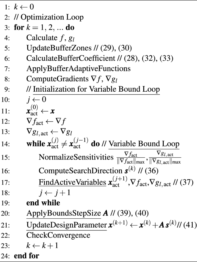
The relaxed gradient projection algorithm (Antonau et al. 2021) is an established method in the industry, which has been designed specifically for large-scale constrained shape optimization problems using Vertex Morphing, as mentioned in Sect. 2.1. It improves the convergence behavior and mitigates zigzagging behavior by using information from previous iterations to create a critical activation or buffer zone around the constraint limit. General formulas are presented briefly below. The interested reader may find a detailed explanation in Antonau et al. (2021). The buffer coefficients of each constraint at optimization step k are computed via:
where is a lower boundary of the buffer zone, is the buffer size, and is the value of the buffer zone’s center. is determined by using the maximum change of the constraint value during optimization:
The computation of and is stated as “UpdateBufferZones” in line 5 of Algorithm 1. Buffer size factor BSF and central buffer value have to be defined initially and may be changed during the optimization. A comprehensive description can be found in Antonau et al. (2021). This buffer adaption is line 7 of Algorithm 1 (“ApplyBufferAdaptiveFunctions”). Buffer coefficients are divided into a relaxed and correction term , which aligns with the original idea of Rosen’s gradient projection (Rosen 1961) to handle non-linear constraints:
where is the initial buffer size factor, and is the maximum correction coefficient (usually ). These calculations are line 6 of Algorithm 1. The search direction is computed from the relaxed projected direction in scaled form:
where is the matrix containing the active constraint gradients in column form, is a diagonal matrix with on its diagonal, and is a vector containing the buffer correction coefficients.
We amend the algorithm by a bound projection method. We follow the steps regarding optimality conditions of bound-constrained optimizations according to Arora (2017). The main idea is to split the design variables into an active set and an inactive set . The algorithm is only permitted to change the active variables. We determine these sets and the resulting feasible search direction iteratively. In the first iteration, all design variables are designated to be active. At the start of each bound iteration , the objective and constraint gradient vectors of the active design variables are scaled by the max norm, and the search direction is computed as in the original method. After that, the new active design variables are found. A variable is set to be active if it is not violating the bounds or it reached the bound, but its search direction shows in the feasible direction:
From there, the loop is continued until the active design variables do not change anymore. The pseudo-code of the iterative computation is shown in Algorithm 1 from lines 9 to 19.
To ensure that not only the search direction obeys the variable bounds, but also the variable update, the step size has to be checked. In this work, we avoid line search techniques and focus on a fixed step size due to the challenges of node-based shape optimization explained in Sect. 2.1. Given a step size , it has to be verified for each design variable that the update
of optimization step does not violate the bound constraints. By limiting the step size for each design variable separately:
a diagonal step size matrix can be formed:
which guarantees that the design variables always stay inside the feasible domain. The pseudo-code of the modified relaxed gradient projection algorithm considering variable bound constraints is given in Algorithm 1 below. The modifications of the original algorithm are marked by underlining. The buffer computations in lines 5 to 7 are not altered from the original algorithm.
Relaxed gradient projection with bounds
The implementation of the same modification for Rosen’s gradient projection algorithm (Rosen 1960, 1961) on which the relaxed gradient projection is based, is straightforward.
Threshold projection functions, as in Yoon and Kim (2003) or Wang et al. (2011), could be used to include bounds instead of our proposed bound projection. However, we aim to develop a bounding method that allows intermediate thickness design variables. Applying threshold projection mapping pushes the variables to their bounds and removes sensitivities once they reach the bounds. As a consequence, they cannot be updated by the algorithm anymore and remain at the bound. This behavior is particularly undesirable in our proposed concurrent shape and thickness optimization framework, which solves a complex, non-linear, and non-convex optimization problem and hence may require that thickness variables can go away from the bounds again.
The subsequent example demonstrates the advantage of applying the variable bounds directly on the design control variables with the modified relaxed gradient algorithm over bound constraints formulated on the physical thickness variables .
2.3.1 Thickness filtering example shell optimization
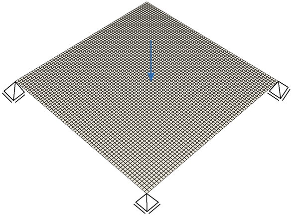
This shell optimization example is adapted from Geiser et al. (2024). A symmetric shell structure, supported at four nodes, one fixed and three roller-supports, similar to a simply supported beam, is loaded statically in the symmetry plane. It is discretized by a regular symmetric mesh with quadrilateral elements (Fig. 3).
We want to minimize the mass while the linear strain energy shall not exceed the value of the initial design . The complete thickness field of the shell is selected as the design variable, and hence, there are as many design variables as nodes. A linear filter is used with radius mm, covering at least six elements. Initially, the shell thickness is a constant field ( mm).
Symmetric shell geometry with four node supports and line loading, regularly discretized
Shell thickness bounds are mm and mm.
We compare three optimization setups:
- (i)First, the bound constraints are formulated on the physical thickness variables:
(42)(43)
leading to a non-linear constraint and interdependency when transforming them from the physical to the design control thickness variables by filtering. The constraints are aggregated by a p-norm method () to reduce the number of constraints, like in Geiser et al. (2021). Because no information about the design control thickness field is necessary, the updated filtering approach is applied. This optimization problem is solved with Rosen’s gradient projection algorithm (GP). To distinguish this strategy from the others, we will refer to it, in this example, as updated filtering.
- (ii)Secondly, Rosen’s gradient projection algorithm is being modified by taking into account linear variable bounds for the design control thickness variables with the introduced initial filtering as mentioned above.
- (iii)And lastly, the results of the relaxed gradient projection algorithm (RGP) with design control thickness bounds and initial filtering are shown.
We apply a constant step size in all cases. The search direction is scaled by the norm such that the maximal design control thickness update can be mm. The step size might be smaller in an optimization step if it has to be limited due to the variable bound. All optimizations are carried out until 100 optimization steps are reached.
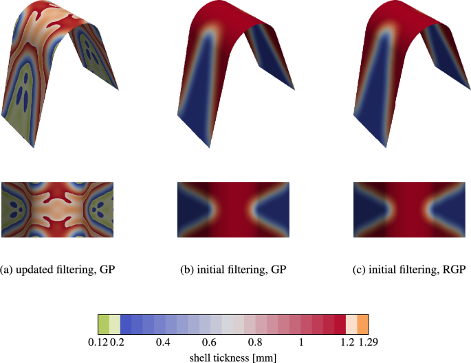
Final shell thickness with the color plot for the three optimization configurations. Isometric view (top) and top view as a 2D projection (bottom)
Final shell thickness designs are displayed in Fig. 4. Both optimizations with initial filtering find almost the same symmetric thickness design and satisfy the variable bound constraints perfectly, see Figs. 4b, c. In contrast, Fig. 4a shows that updated filtering overshoots the bounds and does not yield a symmetric thickness distribution. How much both bounds are exceeded throughout the optimization is plotted in Fig. 5. Again, thanks to the modification of the projection algorithms, the shell thickness is limited flawlessly in the case of initial filtering.
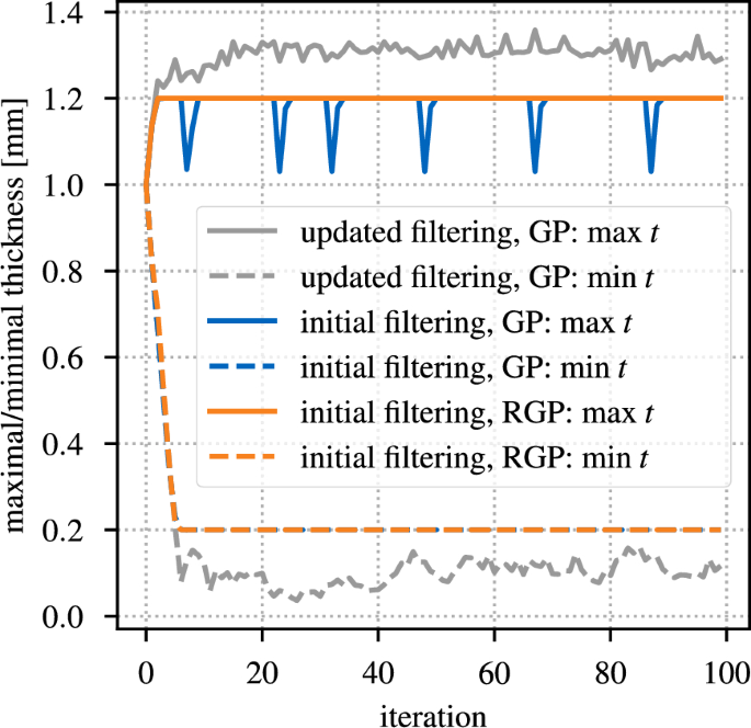
Minimal and maximal shell thickness through the optimization
The superior convergence of the relaxed gradient projection can be viewed in Fig. 6. It mitigates the zigzagging behavior of Rosen’s gradient projection and follows the strain energy constraint boundary better, resulting in smaller constraint violations throughout the optimization, see Fig. 7. Updated filtering violates all constraints, variable bounds, and strain energy (0.83% violation), which results in a mass improvement of 30%. The two initial filtering optimization runs yield a mass reduction of 28%. Yet, just the relaxed gradient projection delivers an entirely feasible design, and the gradient projection algorithm’s design is very lightly infeasible with a strain energy violation of 0.21%.
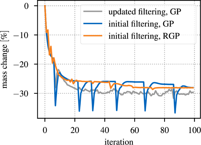
Convergence graph for the mass improvement
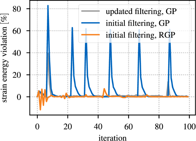
Strain energy constraint violation through the optimization. Negative values indicate no violation
It is worth noting that the final thickness distributions show a clear trend to either the or , similar to results achieved from topology optimization via SIMP. Every design control thickness variable has reached either the lower or upper bound. This binary distribution is intrinsically motivated: the mechanical behavior of the structure is heavily bending-dominated. The thickness has a cubic influence on the bending stiffness of the linear shell element (L S D Morley 1971; Richard H. Macneal 1978) and a linear influence on the mass. This results in a penalization of intermediate thickness values (Cervellera et al. 2005), similar to the penalization of the stiffness term in the SIMP method. That is why the optimization algorithm is encouraged to assign as much thickness as possible to the areas of high bending moments and remove it otherwise. The length scale of intermediate values is equal to the chosen filter radius. Consequently, the thickness filter radius controls the minimum length scale of the minimal and maximal thickness regions. Filtering guarantees a smooth thickness distribution, which is a critical feature in some applications, such as high-pressure die-casted structures. For not bending-dominated structures, intermediate thickness values can be obtained. A Sigmoid function projection might be used to avoid intermediate values in all cases and enforce a black-white design like in Papoutsis (2023).
3 Variable scaling
This section introduces two variable scaling methods. The first improves the convergence behavior of the concurrent shape and thickness optimization with the relaxed gradient projection algorithm. Secondly, the variable scaling technique by Geiser et al. (2024) is adjusted for initial thickness filtering to eliminate discretization-dependent thickness updates.
3.1 Scaling for concurrent optimization
Mechanics of thin-walled structures are built upon the fundamental that the thickness is much smaller than the size of their midsurface geometry. For example, the technical shell theory requires a thin shell with a slenderness of at least , where R is the radius of curvature. Therefore, optimizing both variable types concurrently means that two different orders of magnitude are handled. This influences the second derivatives of the response functions for both the objective and constraints. Gradient-based methods generally struggle with that, particularly if no second-order information is explicitly known or used; large oscillations occur, and lots of iterations are required to find the solution (Arora 2017).
Variable scaling is applied as a means to diminish this effect. We set up a diagonal scaling matrix at the start of the optimization, defining the relation between the physical shape variables, , and , and their scaled counterparts, , and :
where and are diagonal scaling matrices, each created from a single scaling factor:
Variable scaling is consistently incorporated into the Vertex Morphing filtering procedure by applying the scaling matrix to the forward and backward mapping operation:
where is the filter matrix for the combined shape and thickness variables:
Both variable types are scaled concerning their typical update size: either the magnitude of an update in one optimization iteration or the total variable change over the whole optimization. The thickness scaling factor can be computed from the limits:
where is a parameter controlling how many optimization steps it takes to shift from one variable bound to the other. The shape scaling factor can be determined by an appropriate shape update in one optimization step based on the average element size and a user-defined control parameter :
or, alternatively, the axes of an object-oriented bound box around the geometry could be used with a user-defined parameter to estimate the total expected shape change:
If we scale the variables according to their total variable change using (51) and (53), only the parameter must be defined by the user. However, many industrial optimization problems include geometrical constraints limiting the realizable shape design space, so the maximal possible shape change is actually a priori known and can be used as a fitting value for . We may also interpret selecting a suitable shape scaling factor as a conscious decision of how much total shape update is preferred. The concurrent shell example optimization in the following section demonstrates that smaller shape scaling factors lead to designs with less shape change. Multiple other approaches to finding appropriate scaling factors are possible. However, what changes the existent but unknown second derivatives of the response functions is the relation between both scaling factors. A considerable advantage of the proposed scaling method is that no explicitly determined second-order information is required, which would be very costly and generally unavailable for node-based shape optimization. Due to the proposed variable scaling method, we can select suitable values for the step size to update the design variables in a range between around 0.01 and 1.0. In contrast to the method proposed by Papoutsis (2023), the variable scaling technique is computed once at the start of the optimization and does not impose updates of fixed magnitude on both variables in every iteration step. The positive effect on the convergence as a consequence of variable scaling is shown in the following example.
3.1.1 Concurrent optimization shell example
The same arch-like shell structure is optimized as in Example 2.3.1, but this time shape and shell thickness are taken as design variables. Once more, mass is minimized, and the linear strain energy is not allowed to be greater than the initial design. The shape is controlled via a Gaussian kernel with radius mm in an updated filtering manner, except for the surface edges whose positions and tangents are fixed by the damping technique introduced in Baumgärtner (2020). The thickness parameterization and thickness bounds are chosen as above.
The goal of this study is to show the effect of variable scaling. To this end, optimizations without variable scaling are compared to different setups of scaling factors. A step size of is used on the scaled search direction. Because the unscaled optimization does not converge with this step size, it is also increased to in this scenario. All optimizations are conducted with the relaxed gradient projection algorithm. Geiser et al. (2024) showed that an unconstrained shape optimization of the structure is able to achieve a strain energy of just Nmm, which is an improvement of over 99%. For this reason, we may expect to converge to a local minimum with a thickness distribution equal to the lower bound limit mm. This is equal to a mass improvement of at least 80%. In order to compare the convergence behavior, this prediction is used as the exact criteria to stop the optimization.
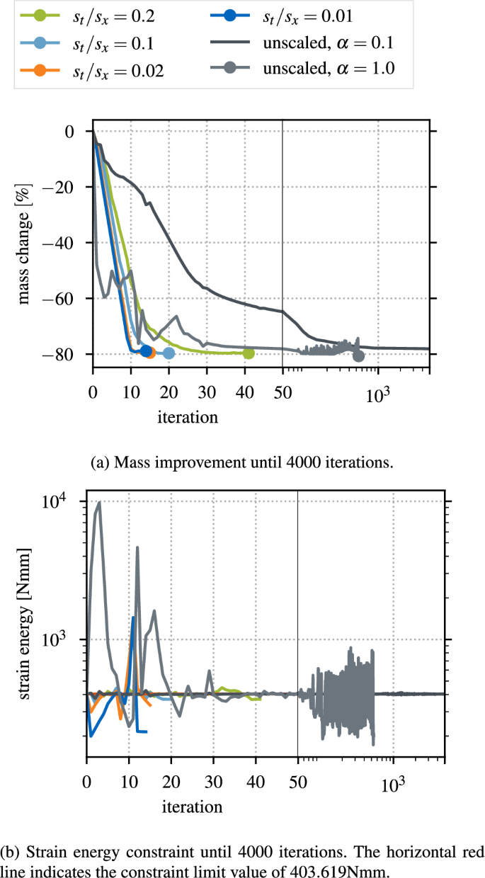
Convergence graph of the mass improvement and strain energy constraint through the optimization. The x-axis changes its scale at iteration 50 from linear to logarithmic
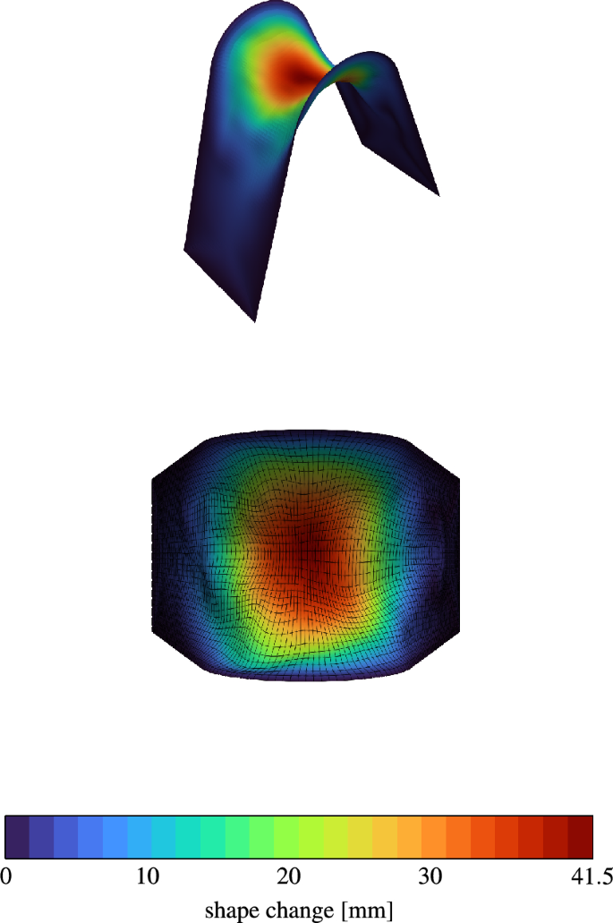
Final shell design with color plot of the shape change in case of the unscaled optimization with step size . Isometric view (top) and top view (bottom)
Figure 8 shows an immense reduction of optimization iterations to reach a global minimum for all scaling factors compared to the unscaled variants. While the unscaled optimization run with a step size of cannot converge in 4000 iterations, the larger step size still requires 540 steps to converge. In both cases, this is impractical for the application, as more complex geometries and optimization problems will require considerable computation time. Even though the mass is reduced very quickly for the unscaled run with a step size of , the strain energy constraint is extremely violated in this optimization phase. Oscillations in the mass graph occur in the first optimization steps and after around 100 iterations. At this time, the mesh deteriorates, which makes the quality of the numerical solution of the physical problem questionable and leads here to an asymmetric shape. The distorted grid of the converged result is shown in Fig. 9.
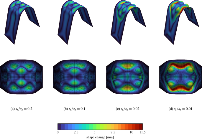
Final shell designs with color plot for different scaling factor ratios. Isometric view (top) and top view (bottom)
Variable scaling for concurrent optimization yields feasible, symmetric, converged shell designs with minor shape changes. Increasing the shape scaling factor accelerates the convergence but comes at the cost of slightly losing mesh quality as more extensive shape updates are provoked. The relation , in combination with the step size of , results in a possible shape update of 5 mm, which is at the limit of a recommended maximum value of r/4 for Vertex Morphing. Larger factors induce less shape change with less distorted grids, which is demonstrated in Fig. 10, still within a superbly low amount of optimization iterations. All shell designs in Fig. 10 have reached the convergence criteria, such that the thickness field equals the minimum thickness of mm.
We can conclude that applying variable scaling influences the convergence positively, leading to designs within a viable time frame. Different local minima are found with different scaling factors due to the non-convexity of the optimization problem.
3.2 Discretization-independent initial filtering
Geiser et al. (2024) has introduced a variable scaling technique to eliminate grid-dependent optimization results for the Vertex Morphing method. The technique revolves around a design variable transformation based on sensitivity weighting, consistently integrated into the Vertex Morphing scheme. We first give an overview of the method in the context of updated filtering and then work it out for the initial thickness filtering process. Discrete design control gradients are obtained from the continuous physical gradients or the continuous design control gradients (Bletzinger 2017):
and so the mass matrix of the morphing functions is the key to deriving the continuous gradients:
Instead of applying the full mass matrix, it is necessary for the case of Vertex Morphing though to use the diagonal mass matrix , as the filtering effect would be removed otherwise. This can be shown by weighting the design control sensitivities by the full mass matrix, applying a steepest descent step:
and filtering the design control update forward:
where the relation with the mass matrix of the discrete shape has been used, which is obtained by solving the integral numerically on the discrete shape (Geiser et al. 2024).
The design variable transformation to the continuous variable spaces is carried out by dividing the inverse diagonal mass matrix into two diagonal scaling matrices :
which are then employed consistently in the backward and forward filtering procedure:
where are the scaled design control variables.
The filter functions of the initial filtering approach are computed on the initial configuration. Hence, we must reformulate the morphing functions’ mass matrix accordingly. The starting point for that is the relation between the discrete and the continuous gradients in Eq. (54). The integral is transformed to the initial configuration by:
where is the area change of the surface. The diagonal mass matrix is now recognizable as:
With this diagonal mass matrix, the scaled thickness variables can be determined in the same way as the scaled shape variables above. The effect of weighting the sensitivities with the proposed diagonal mass matrix for initial filtering is presented in the subsequent example.
3.2.1 Sensitivity weighting example sphere
We examine the mass gradients with respect to the thickness variables and the resulting thickness update with a step size of through two steps of shape deformation, see Fig. 12. As the material density is chosen as , the mass response function equals a volume response function, for which the analytical continuous thickness gradient field is uniformly equal to one (). Weighting the filtered gradients by the inverse of the diagonal mass matrix of (65) should yield the same uniform field equal to one. Additionally, the continuous thickness gradient is invariant to shape changes, so its approximation by the proposed diagonal mass matrix should stay constant through shape deformation. If the sensitivity weighting is well defined, the thickness update should be uniform with an magnitude equal to the step size , which is obtained after the forward filtering of the approximated continuous thickness gradient.
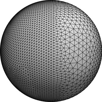
Sphere with irregular discretization (ratio 1:2)
An irregular discretized sphere with radius is studied (Fig. 11). The average edge length of the triangular elements on the left half is 0.43 and on the right 0.86, so in total, there is a ratio of 1:2. Shape change is enforced to form an ellipsoid out of the initial sphere by applying shape sensitivities of and a step size for the shape update of . That changes the size of each element individually and relative to each other and will, therefore, show the effect of discretization-dependent results well.
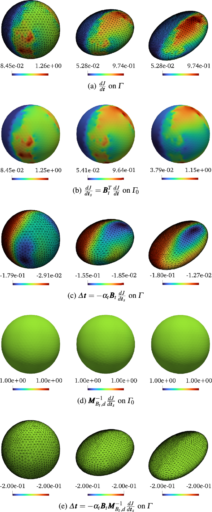
Sensitivity fields and updates of the thickness variables through two steps of shape deformation (from left to right)
The discrete thickness sensitivities are determined on the current geometry by finite differences (Fig. 12a). Filtering on the initial configuration without variable scaling shows an extreme discretization-dependent sensitivity field in Fig. 12b, which causes a smooth but also highly irregular thickness update after the forward filtering (Fig. 12c). On the other hand, using the above proposed diagonal mass matrix for sensitivity weighting, the accurate uniform continuous gradient field with magnitude 1 is obtained, see Fig. 12d. This yields a discretization-independent uniform thickness update after the forward filtering as well (Fig. 12e).
Further studies on grid-independent filtering on the initial geometry configuration are out of the scope of this paper. The interested reader finds an in-depth analysis of discretization-independent shape optimization with the explicit Vertex Morphing method in Geiser et al. (2024). In addition, a transformation of the variable bounds from the non-scaled design control space to the scaled design control space would be necessary to incorporate the discretization-independent initial filtering into the presented shape and thickness optimization scheme. This is not conducted here.
4 Numerical experiments
In this section, various simultaneous shape and thickness optimizations are presented. The first two examples are taken from the literature to compare results from other methods. Lastly, a problem of industrial importance is investigated. Linear static analysis and adjoint semi-analytic sensitivity analysis is conducted with the open-source FE software package KratosMultiphysics (Dadvand et al. 2010) for all examples.
4.1 Simply supported plate
This optimization problem is adapted from Kamper and Naets (2024), who introduced a combined shape and topology method. The structural properties are identical to those of the original problem (Table 1).
Initially flat shell structure
An initially flat, square plate structure is simply supported at its four corner points and loaded in the center (Fig. 13). We also try to reconstruct the optimization problem as closely as possible.
The goal is to minimize the strain energy while reducing the mass to at least 56% of the initial mass. The relation between the mass of the current design and the initial design is also called mass fraction . Shape design variables are restricted to move in the positive -direction and limited to a change of 0.5m. To imitate topology optimization, the lower thickness bound is set to a low value of m. Radii for shape and thickness filtering are set to m. The optimization with scaling factors and is stopped after 200 iterations of a step size of .
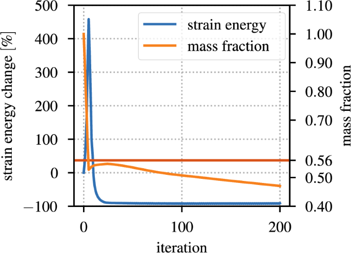
Simply supported plate: strain energy and mass fraction constraint through the optimization. The horizontal red line indicates the constraint limit value of 0.56
With all constraints satisfied, an improvement of 93.28% is achieved; see Fig. 14. Fig. 15 shows a comparison between the concurrent shape and topology optimization of Kamper and Naets (2024) and our proposed concurrent shape and thickness optimization method. Clear x-shaped beads evolve, yielding a final design similar to the study of Kamper and Naets (2024) (Fig. 15a). It is visible in Fig. 15b that just a tiny area at the center reached the upper limit of the shape change. This local constraint violation slows down the optimization significantly. It is conceivable that this would be resolved by applying the initial filtering concept with the modification of the relaxed gradient projection for variable bounds for the shape variables as well.
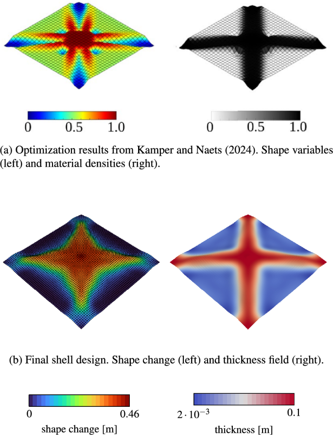
Simply supported plate optimization results. Comparison of the concurrent shape and topology optimization of Kamper and Naets (2024) (top) and our proposed concurrent shape and thickness optimization method (bottom)
4.2 Cowling
The following cowling structure was shape optimized by Firl et al. (2013), and with this design, Arnout et al. (2012) conducted a parameter-free thickness optimization. Träff (2023) used it most recently for a concurrent shape and thickness optimization method. In order to draw up a comparison, the structural properties (Table 2), geometry, boundary conditions (Fig. 16), and the optimization problem are constructed as close as possible from there.
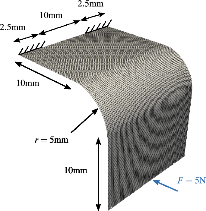
Cowling structure
The objective function is the strain energy. Additionally, a constraint is imposed such that the mass has to be less or equal than the initial mass. All edges of the shell have to remain in their corresponding plane. This is done by damping shape updates normal to the respective plane directions with a radius of mm. Further shape restrictions are not imposed here, as great improvements are already achieved with minor shape changes. A Gaussian shape filter with a radius of mm and a linear thickness filter with a radius of mm are chosen. The thickness bounds are mm and mm. Träff (2023) reached an objective improvement of 99.9% in 400 steps using the MMA, and hence, this improvement is used as the stopping criteria for the optimization. The relaxed gradient projection algorithm is performed with a step size of 0.2 and a scaling factor ratio of .
Cowling: results of shape and thickness optimization of Träff (2023)
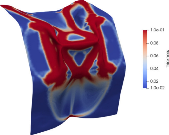
Graphs of the strain energy objective and mass constraint function are presented in Fig. 20. The algorithm successfully converges inside the feasible domain already after merely 50 iteration steps. As mentioned above, just small shape changes are necessary to find an optimal design; see Fig. 18. The free-form parameterization creates an overall complicated shape. However, a v-shaped stiffener is visible from the load point leading up to the middle. Areas of high shell thickness are located in the middle, at the load point, at the supports, and toward them (Fig. 19). The non-convexity of the optimization problem reveals itself when we compare the resulting shell designs of Träff (2023) (Fig. 17) and our proposed method: even though both designs result in almost equivalent objective values, the shapes and thickness fields differ severely. We achieve qualitatively a design with locally lower curvature.
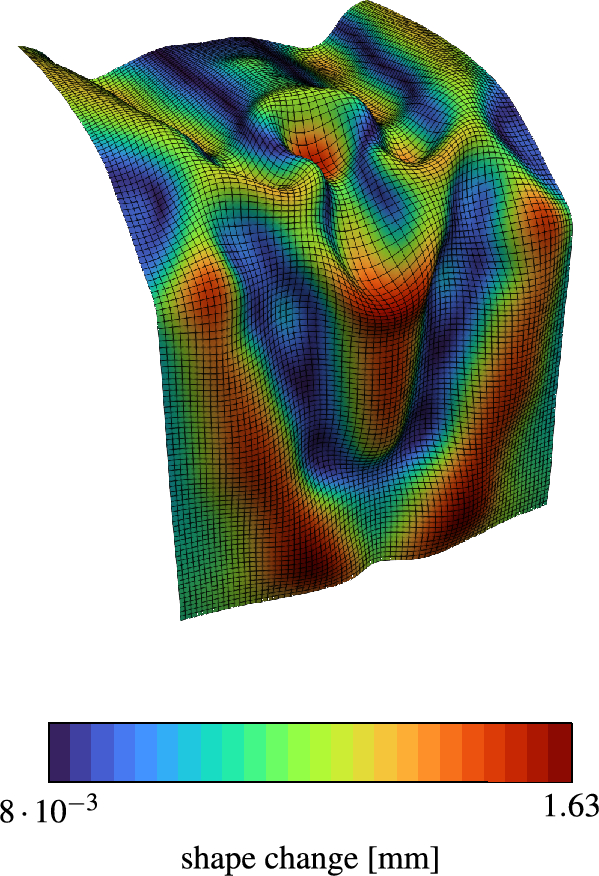
Cowling: final design with color plot of the shape change
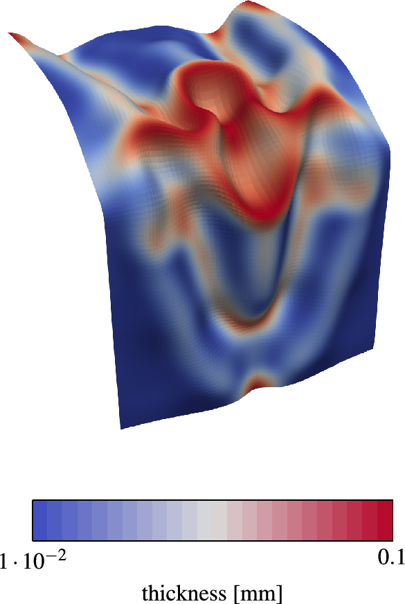
Cowling: final design with color plot of the thickness
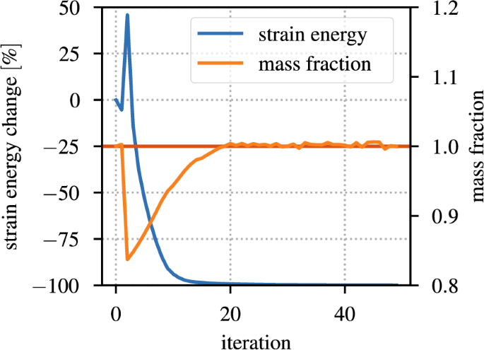
Cowling: strain energy and mass fraction constraint through the optimization. The horizontal red line indicates the constraint limit value of 1.0
4.3 Control arm
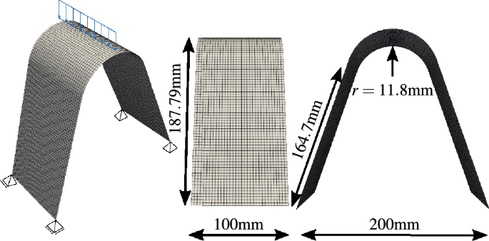
We examine a rough initial design of a lower control arm for an automotive suspension. It regulates the vertical motion of a car wheel due to imperfections of the road surface. Such geometries are often manufactured by high-pressure die-casting, which produces thin-walled structures with varying thickness distribution. A common material for this manufacturing method and lightweight design is aluminum. We choose the properties for the linear elastic material accordingly: Young’s modulus , Poisson’s ratio , and density . The initial geometry and structural problem are displayed in Fig. 21. A vertical force of N on the left side loads the control arm. It is applied as a surface load on the cylindrical hole. Dirichlet boundary conditions are on the right side, which fixes the displacements in all cartesian directions. We discretize the structure by linear triangular shell elements with an average edge length of 2 mm.
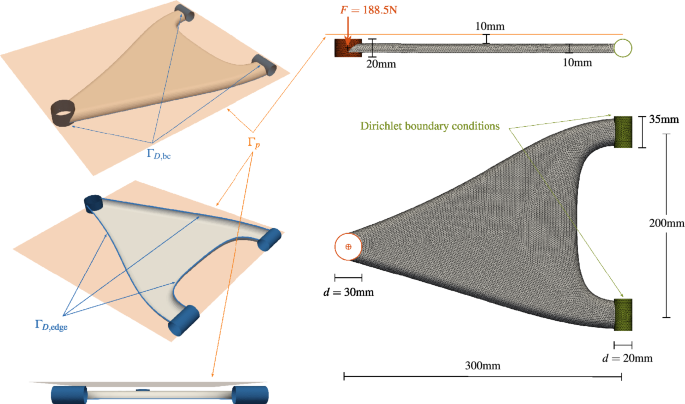
Control arm: initial geometry, structural (right side) and optimization (left side) problem setup
As in the previous examples, the strain energy is the objective of the optimization. The mass should be at least reduced by 25% of the initial design . A geometrical packaging constraint limits the shape design space: the plane , located 10 mm above the design surface, shall not be penetrated. Such design space restrictions are usual for an automotive suspension assembled from multiple parts in a compact space. We apply the node-wise formulation of the packaging constraint for shape optimization from Geiser et al. (2021), where the nodal constraints are aggregated by the p-norm method (). The surface edges are also restrained to remain in their common plane. We achieve this by damping the shape updates in the z-direction at the edges with a radius of mm. The shape of all boundary conditions is fixed as well by damping with a radius of mm in order to keep the connections to other parts of the suspension. Figure 21 depicts the geometrical constraints.
We choose Gaussian filters with a radius of mm for both shape and thickness design variables. The initial shell thickness is mm, typical for aluminum die casting. We define that the optimizer is not able to increase the initial thickness ( mm) and limit the minimal thickness to mm. One hundred steps of the relaxed gradient projection algorithm are conducted with a step size of 0.1 and a scaling ratio factor of .
Figure 22 compares the initial geometry and the optimization result. We identify an increasing height of the shell toward the supports, increasing the second moment of inertia.
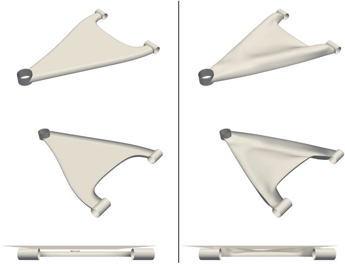
Control arm: comparison of initial (left) and final geometry (right)
A look at the total shape change in Fig. 23 further highlights the creation of stiffeners from the loading area to the supports.
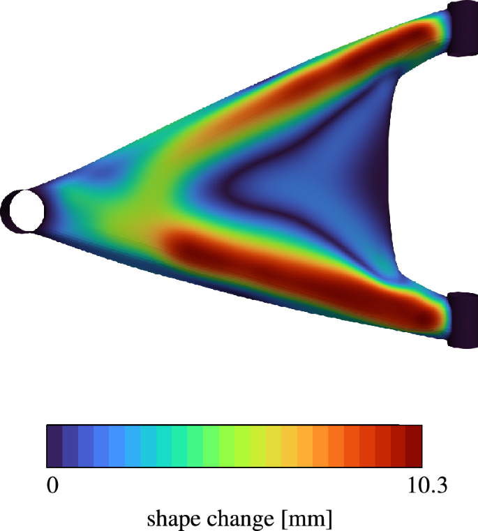
Control arm: final design with color plot of the shape change
The optimization algorithm mostly reduces the thickness in the middle between the two stiffeners and toward the load point; see Fig. 24. These regions are expected to endure smaller internal moments than close to the supports.
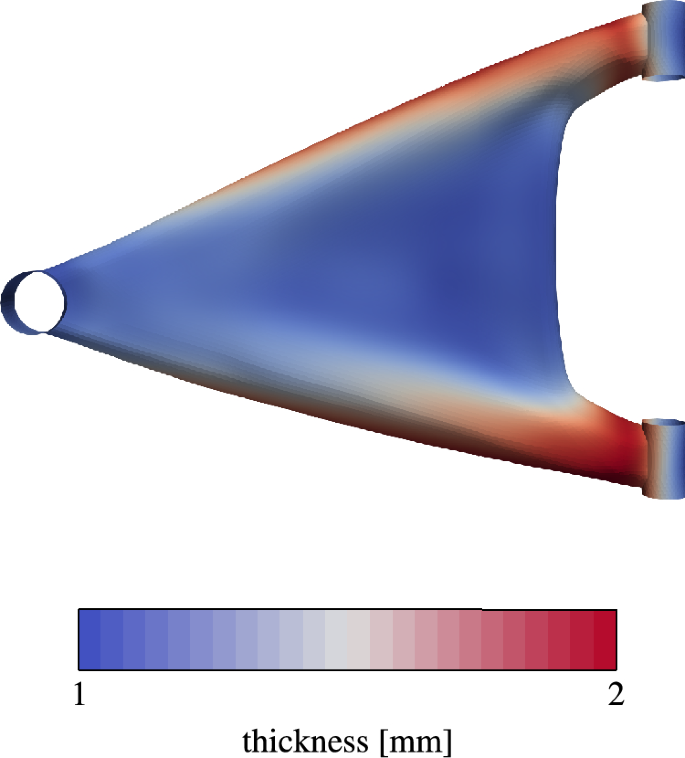
Control arm: final design with color plot of the thickness
Figure 25 shows the maximum penetration of the packaging plane. The packaging constraint is well followed overall, with minor penetrations occurring over the course of the optimization, which is well within a reasonable tolerance.
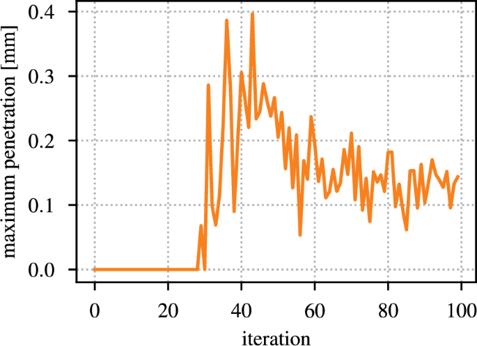
Control arm: maximum penetration of the packaging plane through the optimization
The progress of the strain energy objective improvement and the mass constraint through the optimization is depicted in Fig. 26. The mass constraint is satisfied after merely eight optimization steps and kept in or close to the feasible domain afterward. The final design yields an objective improvement of about 72.7%.
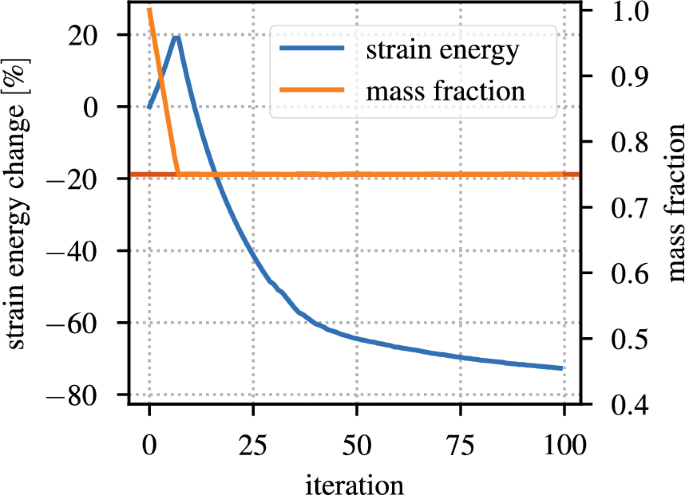
Control arm: strain energy and mass fraction constraint through the optimization. The horizontal red line indicates the constraint limit value of 0.75
5 Conclusion and outlook
A simultaneous shape and shell thickness optimization strategy with the Vertex Morphing method has been presented. For this purpose, the explicit smoothing of the thickness variables has been reformulated such that the filter functions are evaluated on the initial configurations. Thus, a linear relation between the design control field and the physical thickness is maintained. This enables the imposition of bound constraints on the design control variables as they are known throughout the whole optimization process. These thickness variable bounds have been incorporated into the relaxed gradient projection algorithm, allowing it to stay inside the feasible domain in every iteration. Convergence improvements for concurrent optimization have been achieved by suitable variable scaling considering the different physical magnitudes of the two design variable types. The effect of the scaling factor ratio on the result due to the non-convexity of the underlying optimization problem has been highlighted. Additionally, the possibility of eliminating discretization dependencies for the proposed initial filtering approach has been briefly shown by modifying the variable scaling method of Geiser et al. (2024). Further method development on how to translate the variable bound constraint from the non-scaled to the scaled control space is required.
The proposed initial filtering approach, which references variable changes always back to the initial configuration, in combination with the variable scaling, which removes grid-dependent variable evolution, allows the formulation of an explicit filtering technique mathematically consistent with the optimization problem, as it does not alter during the design history. Hence, optimization algorithms may be utilized in a black-box manner. Therefore, it is compelling to apply the initial filtering approach not only to the thickness variables but also to the shape. This would also allow for handling shape bounds elegantly, essential in bead optimization.
A thorough and detailed comparison to the method introduced by Träff (2023) may be attractive due to three aspects: firstly, how the filter choice (implicit or explicit) influences the outcome of a combined optimization. Secondly, which algorithm (MMA or relaxed gradient projection) performs better in this scenario? Lastly, which effect does the element quality constraint have on the regularization, and is it also valuable for the initial explicit filtering approach?