A fiscal equalization scheme needs to balance two conflicting objectives. On the one hand, it has to level out financial resources across jurisdictions. On the other hand, it should not undermine the fiscal incentives for a jurisdiction to improve its own economic position. In Germany’s fiscal equalization scheme, the trade-off between these two objectives is particularly pronounced. First, the combination of comparable expenditure profiles and differing per capita revenues across the 16 federal states provides arguments for a system that levels out diverging revenues broadly. Second, the states have political means to influence and improve their economic and fiscal situation by their own efforts.

The existing literature shows that, in designing their fiscal equalization scheme, the German states solved this trade-off by opting for a highly redistributive system. As a consequence, under this system it becomes fiscally less attractive for a state to maintain and improve its tax base as large parts of the fiscal benefits of such an improvement are redistributed towards the other states and the federal level (see, e.g., Scherf 2007; Fuest and Thoene 2009; Feld et al. 2013; GCEE 2014; Hentze 2015; Buettner and Goerbert 2016; Scherf 2020a, b). Although a high degree of redistribution induces fiscal disincentives, it can still be welfare enhancing to use transfers to reduce disparities between regions, even if it comes at the cost of lower national output (Henkel et al. 2021). Therefore, finding the ideal degree of possibly welfare-enhancing redistribution that reduces disparities, while mainting the states’ incentives to cultivate their tax bases is a permanent challenge. As a consequence, the degree to which the states have chosen equality in revenues over favorable fiscal incentives has not been static over time. Instead, it varied over five major reforms that Germany’s fiscal equalization scheme underwent during the 51 years since its establishment in 1970. Therefore, the fiscal incentives for a state to maintain and improve its tax bases varied with each of the scheme’s reforms.

In this paper, we focus on the fiscal incentives of Germany’s state fiscal equalization scheme and quantify them by calculating each state’s marginal rate of contribution (MRC) to the equalization system in each year since 1970. The MRC reflect the share of a marginal increase in a state’s tax revenues that is skimmed and does not remain in the state, either due to increased contributions to or reduced transfer receipts out of the equalization scheme. To calculate the MRC for every state, we develop a simulation model of the German fiscal equalization scheme for every fiscal year between 1970 and 2021 that considers all relevant revenue sources, all stages of the system as well as each reform of the equalization scheme. To the best of our knowledge, this paper is the first in which MRC of the German state equalization scheme are calculated comprehensively for all years, reforms, equalization stages and revenue sources. This allows us to trace how the fiscal incentives exerted by the scheme developed over time and what effects the scheme’s reforms had on its incentives. The aim of this paper, which is an updated and extended version of a previous paper by Burret et al. (2018), is twofold. First, by including the latest reform of the equalization scheme into the calculations of each state’s MRC, we provide a comprehensive long-term quantification of the fiscal incentives that the scheme and each of its reforms exerted on each state in every year since 1970. Second, we make this comprehensive long-run quantification of the incentives of the German fiscal equalization system accessible for an international audience.

In contrast to our approach, other empirical studies that provide quantifications of the fiscal incentives of Germany’s state equalization scheme calculate MRC based on a selection of revenue sources only (Baretti et al. 2002; Hauptmeier 2007, 2009; Boenke et al. 2017), use single years (Scientific Advisory Board to the Federal Ministry of Finance 2015), ignore repercussion effects of increases in a state’s revenues on the average revenues of all states (Scherf 2020a) or only address the latest reform of the equalization system (Buettner and Goerbert 2016; Scherf 2020a). International evidence on MRC is scarce. Following Burret et al. (2018), Leisibach and Schaltegger (2019) calculate the MRC of the Swiss fiscal equalization system. They report MRC for cantons with high fiscal capacity of between 14 and 21% and for cantons with low fiscal capacity of between 9 and 92%, with an average of 51,4% for the latter in 2019. Canada has a zero percent MRC for provinces with high fiscal capacity and 100% for the provinces with low fiscal capacity (Feehan 2014).

Our results show that MRC have been at continuously high levels. Thus, the system consistently induced unfavorable fiscal incentives for a state to improve its economic position. This is especially the case for transfer receiving states that face an almost full skimming of additional revenues over almost all years. Only the reform of 2005 led to improvements in the system’s fiscal incentives. These improvements have been concealed by the reform of 2020 that pushed MRC to a historic high, inducing a skimming of up to 112% of additional state revenues for some states, meaning that the fiscal capacity of a state after equalization worsens if its revenues before equalization increase.

The remainder of the paper is organized as follows. Section 2 discusses previous findings on the effects of high MRC on the economic and fiscal policy of a jurisdiction. Section 3 reviews the different stages of Germany’s fiscal equalization scheme since 1970. In Sect. 4, we describe our simulation model to calculate the MRC of a state. In Sect. 5, we trace the development of the system’s MRC over the five major reforms which the system underwent. Section 6 concludes.

The incentives that a fiscal equalization scheme exerts on a jurisdiction to improve its economic position can be quantified by the jurisdiction’s marginal rates of contribution (MRC) to the scheme. For a state that contributes funds to the system, the MRC indicate the share of additional revenue that does not remain in the state because of increased transfer payments due to its increased fiscal capacity. For a state that receives funds out of the equalization system, the MRC indicate the share of additional revenues that does not remain in the state due to a reduction of the payments the state receives out of the equalization system because of an increase in its fiscal capacity. Hence, from a theoretical point of view the fiscal incentives for a state to improve its own tax base decrease the higher its MRC are, and the fruits of a growth promoting policy do not remain within the state but are redistributed to other states or the federal level (Koethenbuerger 2002; Buettner 2006; Berthold and Fricke 2006; Bucovetsky and Smart 2006; Feld et al. 2012; Baskaran et al. 2017).

To what extent the concrete incentive effects of MRC influence local fiscal and economic policies in Germany’s fiscal federalism has been analyzed for the municipal and state levels. For the municipal level, Buettner (2006) shows that municipalities in the state of Baden-Wuerttemberg increased their business tax rate after an increase in the MRC of the municipal equalization scheme. Egger et al. (2010) exploit a natural experiment in the state of Lower-Saxony where the municipal equalization scheme was reformed in the year 1999 and confirm the results of Buettner (2006). Egger et al. (2010) argue that the equalization scheme compensates municipalities for the erosion of their tax base due to higher tax rates. Hence, fiscal equalization lowers jurisdictions’ incentives to attract mobile production factors through lowering tax rates. Buettner et al. (2011) find similar results, showing that attempts by the state level to extract fiscal resources from municipalities result in higher tax rates at the local level. Hauptmeier (2007) focuses on expenditure effects for municipalities in Baden-Wuerttemberg. He shows that higher MRC have negative effects on municipal investment spending, measured as a fraction of the overall municipal budget. He argues that it becomes less attractive for a municipality to maintain its tax base through public investment the more the revenues that a municipality can attain from this tax base are skimmed by the equalization scheme.

For the state level, three studies investigate the impact of the equalization scheme’s MRC on state fiscal policies. Hauptmeier (2009) focuses on public expenditures and shows for the period between 1980 and 2003 that increased MRC reduced state spending for infrastructure and education. Baretti et al. (2002) calculate the annual MRC in the German state equalization scheme for the period between 1970 and 1998 and provide evidence that MRC affected state revenues. They show that higher contribution rates to the equalization scheme had a negative effect on the tax revenues of the ten West German states. Following their results, an increase of the MRC of one percentage point reduces a state’s tax revenues relative to GDP by 0.0096 percentage points. Boenke et al. (2017) use a similar framework for the years 1998, 2001 and 2004. According to their results, the tax collection effort of a state is lower, the higher MRC are. That higher contributions to fiscal equalization affects the tax rate set by states is shown by Buettner and Krause (2021). Their results indicate that, in the case of full equalization, states set the rate of the real estate transfer tax 1.3 percentage points higher than without.

All of these studies confirm that high MRC incentivize a jurisdiction to reduce its efforts in improving its economic and fiscal situation and show that, although tax revenues are not a direct policy parameter, the expected changes in tax revenues impact direct policy parameters such as tax rates that are likely to affect a state’s tax base. However, for their empirical applications, the authors only calculate MRC for single years or for limited time periods and do not trace the system’s fiscal incentives over time. Moreover, most of them only consider an increase in the income tax for their calculation of a state’s MRC. Increases of other taxes that are relevant for a state’s contribution to the equalization scheme, such as the corporate tax or the VAT are not considered. Hence, the MRC which are calculated by them tend to be too low. Moreover, for state policymakers it is the overall burden of fiscal equalization which incentivizes their policies instead of focusing on the effects of equalization on single revenue sources only. Given these limitations, this paper, for the first time, quantifies the fiscal incentives of the German state equalization scheme for each federal state and every fiscal year since 1970, while taking into account all relevant revenues and distributive steps of the equalization system and calculating the overall burden that fiscal equalization exerts on a specific federal state.

In Germany’s federalism, the Laender constitute an autonomous federal tier, while the municipalities are an integral part of the state level. To enable the states and their municipalities to fulfill their constitutional tasks, public revenues are distributed towards the different jurisdictions throughout a multi-layered fiscal equalization scheme. This scheme becomes necessary due to two obligations the German constitution (Grundgesetz or Basic Law) sets for the states and the federal government. The Basic Law entitles the states to receive a high enough share of overall public revenues that enables them to fulfill their constitutional tasks (Art. 107 of the Basic Law). Moreover, the Basic Law establishes homogeneous living conditions among all citizens in the federation as a constitutional obligation (Art. 72 of the Basic Law). Thus, the constitution establishes not only an allocative, but also a highly (re-)distributive goal of the equalization system.^Footnote1

3.1 The equalization system from 1970 until 2019

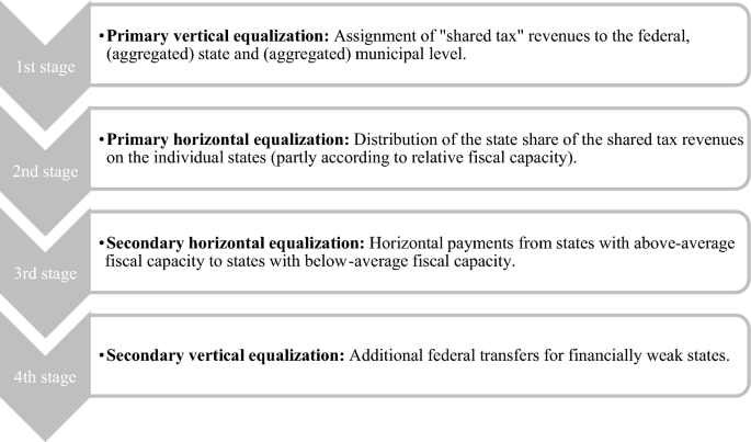
The state fiscal equalization scheme that was effective from 1970 until 2019 comprised four stages. In the first stage, revenues from the so-called “shared taxes” were assigned to the federal and (aggregated) state and municipal levels. These “shared taxes” are the income tax, the corporate tax, the capital (income) tax and the value-added tax (VAT).^Footnote2 Revenues from these shared taxes have been distributed to the (aggregate) state and municipal levels according to fixed shares (see Table 1).

In the second stage of the equalization scheme, the tax shares that had been assigned to the aggregated state level were distributed between the individual states. For the income and corporate tax, this redistribution was based on the tax’s occurrence. For the VAT, up to 25% of the overall aggregated state-share of VAT revenues were assigned to those states that had below-average per-capita tax revenues. The remaining 75% of the state share of VAT revenues were assigned to the states based on their population. Per-capita tax revenues comprised revenues from the income tax, the corporate tax and various state and municipal taxes. As states and municipalities can decide on the rates of some of their taxes autonomously, not actual tax revenues were considered. Instead, imputed tax revenues based on the average tax rates of all states entered the calculation of a state’s tax strength.

The distribution of VAT revenues based on the states’ tax revenues already induced a strong horizontal redistribution of state revenues. Contributing states were those states that were worse-off compared to a distribution of VAT revenues that would have been based on population figures only. This redistributive effect showed up in a change of the revenue ranking for some states. For instance, the state of North-Rhine-Westphalia which had an above-average tax strength before the distribution of VAT revenues arrived at a below-average tax strength after the redistribution of VAT revenues. Thus, it turned from a contributing state in the second stage of the scheme to a receiving state in the subsequent stages of the equalization scheme (Fig. 1).

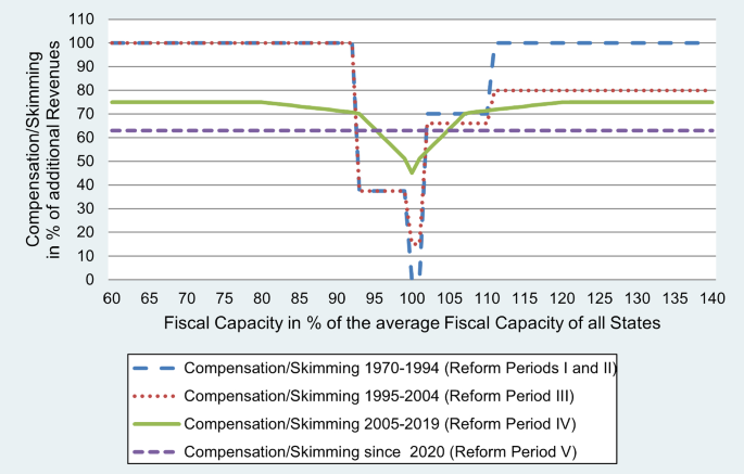
In the third stage of the equalization scheme, differences in per-capita tax revenues were levelled out through horizontal transfers from states with an above-average fiscal capacity^Footnote3 to those states with a below-average fiscal capacity. These transfers were calculated according to a schedule that changed several times since 1970 (see Fig. 2). There were three differences in the calculation of the fiscal capacity of a state in this stage, as compared to the stage before. First, in this stage, revenues from the VAT, from royalties and 64% of municipal tax revenues entered the calculation of a state’s per capita fiscal capacity. Again, not actual revenues from municipal taxes entered the calculation, but imputed revenues based on average tax rates. Second, to consider alleged additional financial needs, the population numbers of the city states Hamburg, Berlin and Bremen were weighted with the factor 1.35, while the population numbers of sparsely populated states were also multiplied by factors greater than one^Footnote4 in order to increase the calculated fiscal needs of these states. Third, since 2005, increases in a state’s per capita tax revenues of up to 12% do not enter the calculation of a state’s fiscal capacity and thus remain within the state of occurrence. This so-called “premia-model” aims at reducing the skimming of additional tax revenues to improve the incentives of the equalization scheme.

The fourth and last stage of the old equalization scheme comprised two sorts of vertical transfers from the federal level to specific states. “General federal transfers” (GFT; Allgemeine Bundesergänzungszuweisungen, ABEZ) were granted as non-earmarked grants to those states that still had a fiscal capacity below 99.5% of the average fiscal capacity of all states after the previous three stages of the equalization scheme. The remaining fiscal gap to 99.5% of the average fiscal capacity was then closed at a rate of 77.5%. In addition to the GFT, the federal government also granted “specific federal transfers” (SFT; Sonder-Bundesergänzungszuweisungen, SoBEZ), independently of the fiscal capacity of a state which aimed to compensate individual states for special fiscal needs.

3.2 The equalization system since 2020

In 2016, the federal government and the state governments agreed to rearrange the fiscal relations between the states as well as between the states and the federal government from 2020 onwards. The two horizontal stages of the equalization scheme described above have been fully replaced by an expanded distribution of VAT revenues that is now augmented by surcharges and deductions based on the per capita fiscal capacity of a state. States with a below average per capita fiscal capacity receive surcharges to their population-based VAT shares, while states with an above average per capita fiscal capacity face deductions from the VAT share that would be assigned to them purely based on their population numbers. Both, surcharges and deductions, follow a proportional schedule that closes 63% of the gap between a state’s per capita fiscal capacity and the average per capita fiscal capacity of all states. With two exceptions, the fiscal capacity of a state is calculated in the same way as in the third stage of the old system. First, municipal taxes are now included into the calculation of a state’s fiscal capacity with a discount factor of 75% instead of 64%. Second, state revenues from royalties are included with a discount factor of 33% only, instead of 100%. Other elements, for instance increased population weights for specific states or the premia model remained parts of the calculation of a state’s fiscal capacity. Vertical GFT from the federal government to specific states also remained part of the equalization system. Those states that still show a fiscal capacity of less than 99.75% of the average fiscal capacity of all states after the VAT distribution continue to receive GFT that close the fiscal gap to 99.75% at a rate of 80%. Note that both, the rate of the schedule and the schedule’s threshold have been increased from 77.5 to 80% and 99.5 to 99.75%, respectively.

As a new element, new SFT have been included into the new system. Those states with municipal tax revenues of less than 80% of the average municipal tax revenues of all states receive vertical transfers (SFT) that, at a rate of 53.5%, close the gap between a state’s municipal tax revenues and 80% of the average municipal tax revenues of all states. Scherf (2020b) argues that these SFT de facto replace former SFT that were granted to East German states to compensate them for politically defined special fiscal needs, independently of their actual fiscal capacity. This new instrument extends the skimming of additional tax revenues to the municipal level. Hence, the new SFT are expected to increase the system’s MRC significantly (Buttner and Goerbert 2016; Scherf 2020b). Besides the SFT for states with below-average municipal tax revenues, the federal level continues to grant additional SFT independently of a state’s fiscal position, e.g., for states with below-average research funding from the federal government.

Although the reform led to major formal changes, there have been hardly any changes that would be substantive to the system’s impacts or to its incentives (Scherf 2020b). Instead, the elements of the old scheme have been transformed into new redistributive instruments. Most of these new instruments are expected to even worsen the incentives the system exerts (Scherf 2020b; Buettner and Goerbert 2016; Feld et al. 2016). However, quantitative evidence on the fiscal incentives of the new scheme is missing so far.

To quantify and trace the fiscal incentives that the equalization system and its reforms exert on the states, we calculate the MRC for each state and year for the period between 1970 and 2021. For our calculation, we set up a simulation model of the German fiscal equalization scheme and use the ex-post data on actual tax revenues. In our model, we use the exact numbers that entered the calculation of the equalization transfers in the respective year for the respective state based on the annual accounts of the Federal Ministry of Finance. Thus, our simulations yield the exact ex-post MRC each state faced in every fiscal year. Note, that the calculated MRC could be endogenous if a state adapts its policy to yield a specific (expected) MRC in the course of the year. This should, however, not cause biased simulation results. The reason for this is that state policymakers can form their expectations on their state’s MRC in year t only on the MRC in year t-1. As the MRC for an individual state within the existing system should however be largely constant, we do not expect that policy changes of a state within a fiscal year are prone to substantially influence the actual ex-post MRC.

Our simulation model is based on a methodology of the German Council of Economic Experts (GCEE 2014) and the existing literature (Baretti et al. 2002; Buettner 2006; Boenke et al. 2017). After replicating the calculation of all equalization payments between the federal level and the states based on the actual revenues of each state in each year,^Footnote5 we apply the following two steps, which are applied separately for each state. First, we ficticiously increase those tax revenues in state A which accrue to the state level. Those are the state shares of the income and corporate tax, the genuine state taxes and municipal taxes. We assume an increase in state A’s tax revenues by a marginal rate of 0.1%, which can be regarded as an increase in a state’s tax base.^Footnote6 Thus, we calculate the average MRC across all state revenue sources. Second, we calculate the marginal retention rate of state A. The retention rate yields the share of the increased tax revenues that remains in state A. We calculate the retention rate as the ratio of the increased tax revenues from state A over the amount of the increase in tax revenues that remains in state A after applying all steps of the state fiscal equalization scheme in order to properly consider all skimming effects. Subtracting the marginal retention rate from one yields the marginal rate of contribution to the equalization scheme.^Footnote7

We set up separate simulation models of the entire equalization scheme for each year for two reasons. First, the absolute and relative contribution rate of a state depends on its relative position among the other 15 states and, thus, on the actual tax revenues of itself and of every other state in each year. Second, we need to recalculate every annual (major and minor) change in the legal framework of the equalization scheme so that our calculations exactly mirror the scheme that was effective each year in every detail. Note, however, that our replication of the fiscal equalization scheme deviates from the actual scheme in one respect. While municipal taxes entered the actual scheme discounted with a factor smaller than one, we include them without a discount factor in our baseline calculations for two reasons. First, in Germany’s fiscal federalism the states are responsible to endow the municipalities with sufficient funds. Thus, for state policymakers the municipalities’ fiscal capacity and their contribution to the equalization scheme is of similar importance as the state’s fiscal capacity itself. Second, the discount factor to which municipal tax revenues were included in the calculation of a state’s fiscal capacity changed several times since 1970. As the factor to which municipal taxes are considered in the calculation of a state’s fiscal capacity directly influences its MRC (the higher the discount factor, the higher the influence of a change in municipal tax revenues on transfer payments) we need to hold the discount factor constant to evaluate the ceteris paribus effects of the reforms of the equalization schemes as well as of each element on the development of a state’s MRC.

Holding the discount factor constant across years yields results that differ from actual MRCs realized by the states. To avoid misleading results of our replication model resulting from differences to the actual fiscal equalization scheme, we run an extension of the simulation model in which we include municipal taxes with the discount factor that was effective in the respective years, thus calculating real marginal effects in addition to the stylized ceteris paribus effects with a constant discount factor. The results of this extension show that actual MRC have been slightly smaller compared to the MRC calculated in our model (see Sect. 6). However, comparing the results of the model with a constant discount factor with those of the model with changing discount factors shows that the replication with constant discount factors is tracing the effects of the different reforms of the schemes on MRC more precisely. Thus, the advantages of holding the discount factor constant described above outweigh the potential drawbacks.

Apart from numerous minor changes, the German fiscal equalization scheme underwent five major reforms since its establishment in the year 1970:

• Reform Period I (1970–1987): Fiscal Reform Act of 1969 and introduction of the horizontal redistribution scheme.
• Reform Period II (1988–1994): Introduction of the GFT.
• Reform Period III (1995–2004): “Solidarity Package I” (integration of the East German states and introduction of the SFT).
• Reform Period IV (2005–2019): “Solidarity Package II” (conversion to a continuous schedule, introduction of a premia model into the calculation of a state’s fiscal capacity).
• Reform Period V (since 2020): General revision of the equalization scheme (elimination of the explicit horizontal stage, expansion of the fiscal capacity based distribution of VAT revenues, introduction of SFT for states with relatively low municipal tax revenues).

Aside the introduction of the GFT in 1988, the periods differ in the applied equalization schedule and in the calculation of a state’s fiscal capacity. Between 1970 and 2004, a discrete schedule was applied. Between 2005 and 2019 this schedule was changed to a linear-progressive one. Since 2020, the horizontal redistribution follows a proportional schedule of the marginal transfer functions as depicted in Fig. 2.

Scherf (2020a) shows that unadjusted MRC can also be calculated without simulating the entire equalization system. Instead of running simulations, he sets up a system of equations to calculate a state’s marginal contributions across the different steps of the equalization scheme. The approach of Scherf (2020a) has the advantage that a complicated simulation of the whole system is no longer needed. Moreover, his system of equations allows the observation of the skimming effects for single tax sources of states and municipalities. There are, however, two downsides of this approach. First, the approach is easy to implement for the post 2019 system with a proportional schedule and without the complicated two-stage horizontal redistribution of revenues that was effective before 2020. Second, his approach ignores repercussion effects of a single state’s increased tax revenues on average tax revenues of all states. Thus, his approach overstates MRC compared to effective marginal contributions to the equalization system.^Footnote8