Nowadays, there is an ever-growing number of applications in which nonlinearities are exploited for functional purposes rather than avoided. These applications include frequency division (Qalandar et al. 2014), vibration mitigation (Bellet et al. 2010), nonlinear energy sinks, and targeted energy transfer (Vakakis et al. 2022). Other applications can be found in micromechanical sensors (Zhang et al. 2002; Marconi et al. 2021a).

Therefore, this increased interest in nonlinear dynamics has favored the development of different numerical methods in the field of reduced order models (ROM, Tiso et al. 2021; Touzé et al. 2021) to analyze and study the nonlinear dynamic behavior of mechanical systems. This behavior can be described through the nonlinear frequency–amplitude relation, which can be tracked by computing the backbone curves (see, e.g., Breunung and Haller 2018). Usually, these curves are obtained using numerical continuation techniques with the collocation method (Dankowicz and Schilder 2013), the Harmonic Balance Method (HBM, Krack and Gross 2019), or the shooting method (Kerschen et al. 2008). Alternatively, the conservative backbone curves can be computed using the reduced dynamics on Lyapunov Subcenter Manifolds (LS^Footnote1), which has proven to be particularly effective for high-dimensional mechanical systems (Jain and Haller 2022).

However, despite all these techniques, controlling the nonlinear dynamic behavior of a system still remains a complex challenge. The main difficulty is identifying the ideal set of parameters that will produce the desired frequency–amplitude relation. To address this issue, various optimization strategies have been proposed. For example, Schiwietz et al. (2024, 2025) used shape optimization to optimize the eigenfrequencies and the modal coupling coefficients of a geometrically nonlinear MEMS gyroscope, whereas Detroux et al. (2021) focused on tailoring backbone curves using nonlinear synthesis. Dou et al. (2015); Dou and Jensen (2015, 2016) developed methods to optimize hardening behaviors in resonators and plane frame structures via nonlinear normal modes (NNMs, Kerschen et al. 2009; Haller and Ponsioen 2016) and the HBM. Incidentally, we notice that in all these parametric optimization methods, the considered structures are of low dimension, usually featuring 2D beam elements and frame-like structures. However, computational times are usually omitted, making it challenging to assess their efficiency and scalability.

These optimization processes are highly sensitive to user-defined parameters, such as the number of harmonics in the harmonic balance method (HBM) or the arc-length parameter in numerical continuation, which may require adjustment during iterations due to changes in system behavior. Additionally, intrinsic limitations of the numerical method, particularly in HBM sensitivity analysis, may affect the optimization results (Saccani et al. 2022). One way to mitigate this issue is by employing alternative methods for computing the frequency–amplitude relation.

Recently, a parametric optimization approach was proposed to tailor the conservative backbone curve^Footnote2 of nonlinear mechanical systems by exploiting the reduced dynamics on the LS (Pozzi et al. 2024). In that work, we highlighted several advantages of the LS’s analyticity in optimization, such as eliminating the need for user-defined parameters, simulations, or ROMs. However, the sensitivities are still computed via direct differentiation, which is computationally demanding as the number of optimization parameters increases.

Despite these advancements in nonlinear dynamics optimization, the available methods in the literature remain applicable only to small systems due to the high computational costs and limited scalability. As a result, topology optimization techniques (Bendsøe and Sigmund 2004), which involve a large number of design variables, are predominantly applied in the realm of linear structural dynamics (Silva et al. 2019; Li et al. 2021; Pozzi et al. 2023b), with applications extend to mechanical resonators (Yang and Li 2013, 2014; Pozzi et al. 2023a; Giannini et al. 2024), MEMS gyroscopes (Giannini et al. 2020, 2022), and piezoelectric energy harvesters (Townsend et al. 2019).

As previously discussed, nonlinear dynamic topology optimization is extremely resource-intensive. To address this challenge, studies such as those by Kim and Park (2010); Lee and Park (2015); Lu et al. (2021) have employed the Equivalent Static Load method (ESL, Choi and Park 2002). This approach converts the nonlinear dynamic problem into a linear static problem. Following a different approach, Dalklint et al. (2020) introduced a topology optimization method for finite-strain hyperelastic structures, incorporating lower bound constraints on the nonlinear eigenfrequencies. These eigenfrequencies are evaluated around the equilibrium configuration, which is determined by solving a nonlinear stationary problem. Similarly, Li et al. (2022) proposed an eigenvalue topology optimization problem with frequency-dependent material properties.

However, despite these attempts, there are no topology optimization approaches that directly target the backbone curve of nonlinear mechanical systems.

Our contribution

As a first step to this end, we focus on the third-order backbone coefficient, which governs the hardening or softening behavior of mechanical systems. As shown in Pozzi et al. (2024), the most resource-intensive part of this process is the sensitivity analysis. Recently, Li (2024) explicitly derived the sensitivities of third-order spectral submanifolds in mechanical systems using both the direct approach and the adjoint method. As pointed out by Li (2024), the computational performance of sensitivity via adjoint method highly depends on the efficiency of evaluating nonlinearities. Here, we follow the adjoint method as in Li (2024) but utilize the tensor notation (Marconi et al. 2020) to handle nonlinear terms more efficiently. This leads to a more efficient sensitivity expression and enables us to apply standard topology optimization algorithms. We use a density-based approach with the solid isotropic material with penalization scheme (SIMP, Bendsøe and Sigmund 1999). Nonetheless, the sensitivity formulation is also valid for other topology optimization approaches, e.g., the level set method (Wang et al. 2003; Allaire et al. 2004), evolutionary structural optimization (ESO) method (Xie and Steven 1993), and moving morphable components (MMC) method (Guo et al. 2014).

The remainder of the paper is organized as follows. In Sect. 2, we show how to compute the third-order backbone coefficient, denoted by , using the normal-form parametrization of the Lyapunov subcenter manifold. The sensitivity expressions of  are derived in Sect. 3 using the adjoint method. In Sect. 4, we briefly discuss the topology optimization approach that is used to obtain the numerical examples in Sect. 5. Finally, we close with the conclusions in Sect. 6.

2.1 General settings

Consider the following equation of motion for a generic autonomous, undamped, nonlinear mechanical system:

where  is the displacement vector, n is the number of degrees of freedom,  are the mass and linear stiffness matrices, respectively, and  is a displacement-dependent nonlinear term. When considering geometric nonlinearities, in several cases (e.g., for continuum finite elements with linear elastic constitutive law and total Lagrangian formulation), this term can be exactly represented by

where  and  are the quadratic and cubic polynomial terms in the displacements, respectively, representing the internal nonlinear elastic forces.

The linear normal modes (LNM) of the system in Eq. (1) are obtained by solving the generalized eigenvalue problem

where  and  are the eigenfrequency and the eigenvector, respectively, associated with a given LNM, mass normalized as

In the absence of nonlinearities, the term  vanishes, and the system in Eq. (1) becomes linear. In this case, it is well known that a subset of LNM can rigorously describe the dynamics of the system. Indeed, this LNM subset spans an invariant subspace-a lower-dimensional space where any motion that starts within it remains confined to it at all times. Due to this invariance, LNMs provide a basis for modal truncation, a rigorous model order reduction method for linear systems. If we restrict the analysis to a single mode , such a subspace takes the form of a (hyper-)plane, spanned by the two eigenvectors of the first-order system associated with that mode.

In nonlinear systems, and under certain conditions (see Kelley 1969), such a plane can be smoothly extended to an invariant manifold, which is a (hyper-)surface, filled with periodic orbits of the full system and tangent at the origin to the aforementioned plane. A schematic representation of these two constructs is provided in Fig. 1, where it is evident that the linear subspace and the manifold are almost indistinguishable for displacements small enough, but they considerably differ as we depart from the origin. In recent years, the theory of spectral submanifolds (SSMs) has emerged as a rigorous method to identify these manifolds for dissipative mechanical systems and utilize them for model order reduction of nonlinear oscillatory systems. In the conservative and autonomous limit, SSMs coincide with the so-called Lyapunov subcenter manifold (LS), a unique, analytic, two-dimensional nonlinear extension of the corresponding linear subspace.

As discussed in the following, the reduced dynamics on an LS provides an analytic expression for the backbone curve of the corresponding mode. This analytic expression can then be used to derive explicit sensitivities for the optimization problem (Pozzi et al. 2024).

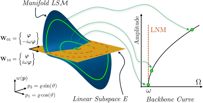
Left: schematic representation of an invariant linear subspace E (yellow plane, spanned by the eigenvectors  and ) and an invariant manifold tangent to it (blue surface). The conservative periodic orbits of the linear autonomous system lying on the linear subspace are drawn in red (dashed line), while the ones of the nonlinear system lying on the manifold are shown in green (solid line). Right: orbit amplitudes and frequencies construct the conservative backbone curve. The LNM is shown for completeness

Full size image

2.2 Model order reduction

We provide here a brief overview of the main steps in model order reduction using invariant manifolds, without discussing the underlying theory in detail. For a comprehensive explanation, refer for instance to Jain and Haller (2022); Thurnher et al. (2024).

Let us assume that the reduced dynamics of a particular mode  of the second-order system in Eq. (1) can be described by  reduced coordinates, collected in a vector . In a linear system, this would correspond to the vector of modal coordinates associated with the same mode (in first-order form), and the linear reduced dynamics would write as

A similar approach can be sought for nonlinear systems using, among other methods, the normal-form parametrization. Letting  be a parametrization of the reduced dynamics, we can thus write:

In linear systems, one would retrieve the full state of the system  as , where  is a matrix collecting the two eigenvectors (see Fig. 1). Similarly, we can retrieve the full displacement of a conservative, autonomous nonlinear system by mapping the reduced coordinates to the LS.

Let  be a parametrization of the Lyapunov subcenter manifold around a (linear) master subspace E. We can write

being  graphically represented as the blue surface in Fig. 1.

Finally, to numerically compute an approximation to  and , and adopting the multi-index notation, we can Taylor-expand them as

where  and  are the reduced dynamics and the manifold coefficients, respectively.

Finally, substituting Eqs. () into Eq. (1), one can solve for the coefficients  and . The procedure to compute them up to the third order is detailed in Appendix A (in particular, see Table 6).

2.3 Backbone curve

Transforming the reduced coordinates into polar notation as , and after some manipulation, it can be shown that the following nonlinear frequency–amplitude relation holds:

where  is the frequency of the response,  is the amplitude in the reduced space, and  are the coefficients of the backbone curve that come from the normal-form parametrization of the Lyapunov subcenter manifold. In particular, if the maximum expansion order is , the backbone curve becomes

where  is the third-order backbone coefficient obtained from the reduced coefficient  at order 3 (i.e., for ).

In this case, the parameter , hereafter renamed  to ease the notation, controls the hardening/softening behavior of the system (Fig. 2, de la Llave and Kogelbauer 2019) and reads (Li 2024):

In the following, only the relevant steps involved in the adjoint sensitivity analysis are reported (refer to Appendix C for more details).

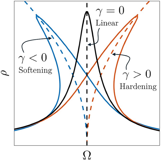
Examples of backbone curves (dashed lines) of the autonomous, conservative systems and of the corresponding frequency response curves (solid lines) for their non-autonomous, non-conservative counterparts, where light damping has been considered

Full size image

The third-order nonlinear force associated with the multi-index  is

The vector  depends on the LS coefficients at lower orders , , , and . These can be computed using the set of equations listed below:

and

and

Remark (On generalization). The results recalled in this section hold for an autonomous, conservative second-order nonlinear system of ODEs. However, LS (and SSM, de la Llave and Kogelbauer 2019) theory holds for generic first-order nonlinear systems of ODEs, therefore extensions to other problems and physical domains are also possible.

When dealing with optimization problems with a large number of design variables, e.g., topology optimization, the sensitivities are usually obtained using the adjoint method. For instance, provided that the mode shape  is mass normalized (Eq. (4), the sensitivity of the eigenfrequency  (Bendsøe and Sigmund 2004) is computed as

Using the same approach, the sensitivity of  is computed using the adjoint method. We follow the derivation in Li (2024) but restrict to the case of undamped system. The state variables of this problem are , , , and . Each of them is associated with a state function (Eqs. (3), (4), (12), and (13)) and with an adjoint variable (, , , and ). Using this terms, the Lagrangian function  is defined as follows:

The adjoint variables are computed by solving the adjoint equations, which are obtained by differentiating  with respect to the state variables:

Equations (19) and (20) are solved together by creating the system

where the terms in the right-hand side are defined as

Finally, the sensitivity of  is equal to the partial derivative of  with respect to the design variables :

where the partial derivatives of the matrices and vectors , , and  depend on the formulation of the mechanical system under consideration. Notice that . This formula is consistent with equation (111) of Li (2024) when damping coefficients  and  in (111) are set to be zero.

All the details on the partial derivatives are given in Appendix C.

The sensitivity expression in Eq. (23) is validated against finite differences perturbing 50 randomly selected elements over the grid used in Sect. 5.1, with different steps :

The small magnitude of the relative error (Fig. 3) confirms the validity of the adjoint method implementation.

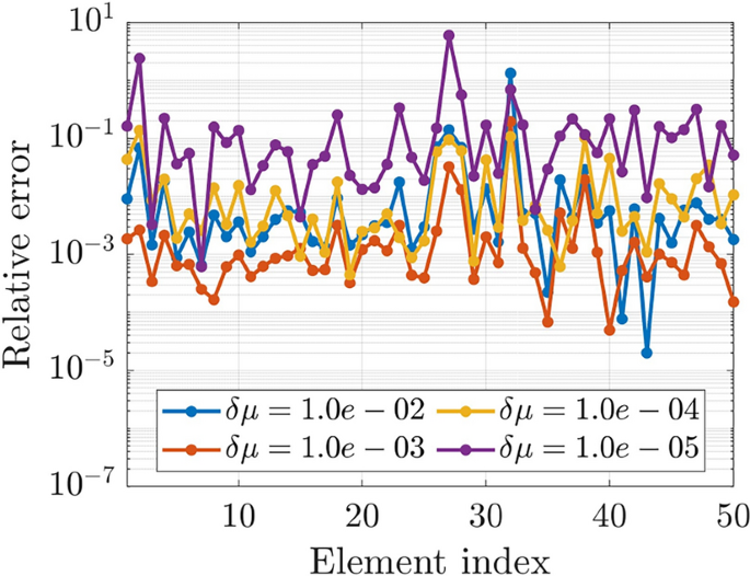
Validation of the sensitivity of  (Eq. (23)) using finite differences

Full size image

In this work, the density-based topology optimization approach is used with the solid isotropic material with penalization (SIMP, Bendsøe and Sigmund 1999) interpolation scheme. As mentioned in the introduction, any topology optimization method can be chosen, and the SIMP choice is dictated only by the ease of implementation in YetAnotherFEcode (Jain et al. 2022). In any case, according to the numerical tests that will be discussed in Sect. 5, topology optimization routines account only for approximately the 4% of the whole iteration computational time. The design domain is discretized using a structured grid made of bilinear squared elements, each one is characterized by density  (Fig. 4).

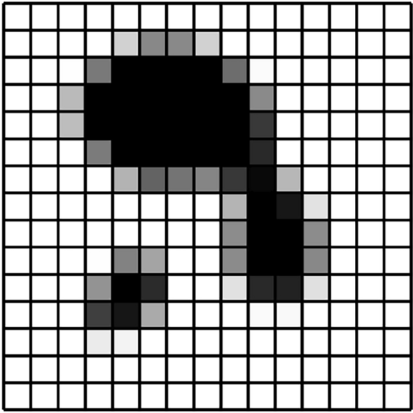
Example of structure discretization using element densities

Full size image

To obtain a well-posed optimization problem, to avoid mesh dependent solutions, and to prevent gray transition regions, the regularization filter described in Wang et al. (2011) is used:

where  is the filtered density of the element e,  is a set that contains the indices of the elements that lay within a circle of radius R around element e, and  is a weight defined as

where  and  are the coordinates of the centroids of elements e and j. In this work,  is used.

The filtered densities are then projected through the projection threshold presented in Wang et al. (2011):

where  is the projected density of element e, and  and  are projection parameters. In this work,  and  are selected.

Finally, the SIMP scheme is used to obtain the physical densities  from the projected ones :

where p is the penalization power, and  is an arbitrary small density of the void element, used to prevent singularities in the numerical method. To ensure a 0/1 design,  is used and p is gradually increased during the optimization starting from 1.

The physical densities  are then used to interpolate the material properties:

where  is the total number of elements,  and  are the quadratic and cubic stiffness tensors, and where we use the subscript e to denote the same entities at element level. The operator  represents the finite element assembly across all the elements of the grid. Since a structured grid is used, the element matrices and tensors are the same for all the elements. Therefore, they can be computed only once and for all, considerably alleviating the total computational cost.

Remark (Nonintrusive implementation). The presented approach employs tensors that are not commonly available in standard FE codes. However, non-intrusive techniques can be used to evaluate nonlinear forces, as demonstrated by Li et al. (2025). While this circumvents the need for tensors, it comes at the cost of losing the previously mentioned advantages. Specifically, in this case, the regularity of the mesh cannot be exploited, as each term would depend on the displacement vector , requiring evaluations to be carried out for every individual element over the entire mesh.

To compute adjoint sensitivities (Eqs. (15) and (23)), partial derivatives of , ,  , and  are required with respect to . This partial derivatives involve differentiating Eqs. (25), (27), and (28). The detailed expressions for these derivatives are provided in Appendix D.

In this section, numerical examples are presented to show the validity of the adjoint sensitivity formulation. In all the examples, the 2-dimensional design domain is discretized using a structured grid made of 4-node, square elements with bilinear shape functions. The material considered is polysilicon (Acar and Shkel 2009), which is characterized by density , Young’s modulus , and Poisson’s coefficient 0.23. The plane stress approximation is used, with a thickness of .

During the optimization, the modal assurance criterion (MAC, Kim and Kim 2000) is used to track the targeted mode, thus allowing to deal with mode switching and to neglect artificial modes that may arise (Pozzi et al. 2023a).

In particular, the MAC value is a measure of the similarity of two mode shapes:

At each iteration, the MAC is used to compare a set of modes with the shape of the target one. This target shape is either known a priori or selected at the first iteration. The mode shape with the highest MAC value is the target one.

The optimization problem is implemented in MATLAB R2023b using YetAnotherFEcode (Jain et al. 2022) and solved with the Method of Moving Asymptotes (MMA, Svanberg 1987).

The most expensive part of the optimization loop is the evaluation of  and its sensitivity, accounting for around  of the total iteration time. Table 1 summarizes these computational times, measured on a Windows laptop with an Intel Core i7-1255U CPU @ 1.70 GHz and 16 GB of RAM @ 3200 MT/s, using different number of elements.

For each example, the optimal layout, the third-order backbone curve in the reduced space (Eq. (8)), and the third-order backbone curve in the physical space are shown. In particular, the latter is computed on the optimal layout using the SSMTool (Jain et al. 2023) at  and  expansion orders.

Remark (ROM accuracy). The presented optimization scheme focuses on , the lowest order nonlinearity coefficient appearing in the backbone curve expression of Eq. (8). As such, we can only guarantee that for a small enough displacement amplitude the dynamic behavior of the system will be of the hardening or softening type, quantitatively determined by the target value of . For high enough amplitudes, the third-order approximation is expected to become less accurate, as higher order terms in Eq. (8) may be required to describe the dynamics of the system.

5.1 MBB beam

The first example is the Messerschmitt-Bölkow-Blohm (MBB) beam with a fixed region ( of the total beam length) in the middle that acts like a proof mass. Thanks to design symmetries, only the left half of the beam is modeled (Fig. 5). The design domain () is discretized using a  grid. A constraint on the maximum area fraction  is used to limit the material usage.

Using these same settings and initial conditions, we set up 3 frequency maximization problems applying different constraints. In all cases, the target frequency  corresponds to the mode shape featuring a vertical oscillation of the proof mass.

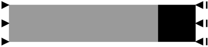
Problem settings and initial conditions for the MBB beam. Only the left half of the structure is optimized. The left side is fixed, while the right side can move vertically but not horizontally. A black region ( of the total beam length) is used as a proof mass

Full size image

The total number of iterations, along with the computational times, for the three examples are reported in Table 3.

MBB—Linear Optimization

First, the following classic frequency maximization problem is solved, with no constraints on :

The optimal layout (left column of Fig. 6) is characterized by a positive , as indicated in Table 2. A positive  corresponds to a material configuration that exhibits hardening behavior, where the structure’s dynamic stiffness increases with increasing deformation.

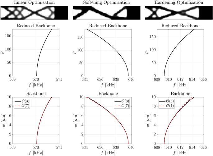
Optimal results of the beam examples (Sect. 5.1). Left column: linear optimization (Problem (31)). Middle column: softening optimization (Problem (32)). Right column: hardening optimization (Problem (33)). The second row shows the third-order backbone curves in the reduced space (Eq.(8)), while the last row shows the backbone curves in the physical space using two different expansion orders

Full size image

MBB—softening optimization

A softening behavior can be obtained including a negative upper bound on the value of . To this end, the optimization problem is recast as

where a  is used, reasonably selected by comparison with the outcome value of  from the previous linear optimization.

The result (middle column of Fig. 6) is characterized by a negative value of , as indicated in Table 2, leading to the desired softening behavior. A negative  implies that the structure undergoes a reduction in stiffness for increasing oscillation amplitudes. Interestingly, in this case, the optimization process converged to an asymmetric layout about the horizontal axis, exhibiting behavior similar to that of curved beams or arches (Marconi et al. 2021b).

MBB—hardening optimization

We now add a positive lower bound to the coefficient . The aim here is to control the hardening behavior of the structure. The optimization problem becomes

where  is selected.

The optimal solution is presented in the right column of Fig. 6. This structure exhibits a positive , indicating the desired hardening behavior. In particular, the value of  is an order of magnitude larger compared to the solution of Problem (31), showing a significantly enhanced stiffness response under deformation (Table 3).

5.2 Single mass MEMS resonator

The second example is a single mass MEMS resonator for high-frequency applications. The design domain () is discretized using a  grid. Problem settings and boundary conditions are described in Fig. 7. The black region represents the proof mass that remains constant for the entire optimization. Fixed boundary conditions are applied to both the left and right sides of the domain.

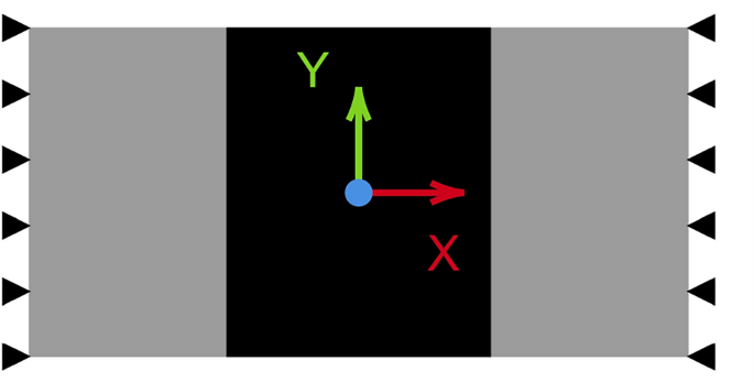
Problem settings and initial conditions for the MEMS resonator

Full size image

The first optimization problem aims at imposing the frequency , which corresponds to the mode shape with the maximum displacement of the proof mass along the Y direction. To avoid material detachment and connectivity issues, a constraint (or the objective function) is chosen to maximize the frequency , which corresponds to the mode shape with the oscillations of the proof mass along the X direction. A constraint on the maximum allowable area is also applied. Again, using these common settings, the optimization is carried out for 3 different cases.

The total number of iterations, along with the computational times, for the three examples are reported in Table 5.

MEMS—linear optimization

The optimization problem is initially formulated without any particular constraint on  and maximizing the objective function :

where  and  is the target frequency value. The value of  represents the relative error of  with respect to . For this problem,  is used, meaning that the constraints is satisfied if the value of  is within  of the target value (between  and ).

The optimal layout (left column of Fig. 8) is characterized by a small positive nonlinear coefficient associated with . This results in an almost linear behavior in the considered oscillation amplitude range.

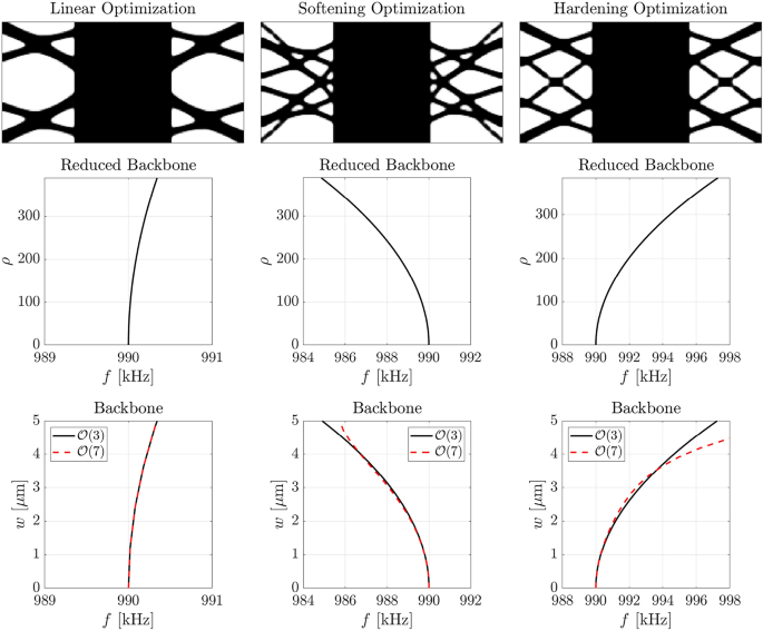
Optimal results of the MEMS resonator examples (Sect. 5.2). Left column: results obtained solving Problem (34). Middle column: results obtained solving Problem (35). Right column: results obtained solving Problem (36). The second row shows the third-order backbone curves in the reduced space (Eq.(8)), while the last row shows the backbone curves in the physical space using two different expansion orders

Full size image

MEMS—softening optimization

Problem (34) is now modified to minimize the coefficient  while imposing the same constraints on the target frequency  and the maximum allowed area. The maximization of  (required to avoid material detachment and connectivity issues) is recast as an additional inequality constraint. The softening optimization problem reads:

where .

The result of the optimization (middle column of Fig. 8) is characterized by a negative value of , as indicated in Table 4, leading to the desired softening behavior.

MEMS—hardening optimization

Finally, Problem (35) is modified to maximize the coefficient :

where all the constraints are the same as in Problem (35).

The optimal solution is presented in the right column of Fig. 8. This structure exhibits a positive  (Table 4), indicating the desired hardening behavior. In particular, the value of  is an order of magnitude larger compared to the solution of Problem (34) (Table 5).

In this paper, we proposed a structural topology optimization method designed to tailor the hardening and softening dynamic behavior of nonlinear mechanical systems. The main advantage of the proposed approach is that it eliminates the need for costly full-order simulations or numerical continuation and significantly reduces the computational effort in optimizing the backbone curve. This reduction is achieved rigorously via analytical expressions for computing the conservative backbone from the reduced dynamics on the corresponding Lyapunov subcenter manifold.

We demonstrated how the integration of the adjoint method for the sensitivity analysis, combined with the tensor notation for expressing nonlinear internal forces, further enhances the computational efficiency of the proposed optimization process, especially for high-dimensional finite element models. The tensorial formulation not only simplifies sensitivity evaluations but, when applied to regular grids of elements, proves highly efficient in terms of computation. Numerical examples have been provided to show the validity of the proposed optimization.

While the current work focuses on third-order expansions and on the coefficient , future extensions could adapt the approach to higher orders and to different optimization targets. Arbitrary order expansions would open up the possibility of adaptive algorithms to control the accuracy of the ROM during optimization, as done in Pozzi et al. (2024). Moreover, the adjoint formulation could be recast in order to optimize directly the backbone or the frequency response curves in the physical space. All these developments are currently underway (Pozzi et al. 2025).