Article Content
1 Introduction
Modeling the stock price processes in the market is a crucial topic. An incorrect or overly simplified evaluation of stock prices can have serious consequences for investors. The standard assumption of asset prices following a geometric Brownian motion can be extended by considering features such as stochastic volatility (see Broto and Ruiz 2004; Asai et al. 2006; Maasoumi and McAleer 2006) or jumps (see Wu 2003; Ceci and Colaneri 2012; Oliva and Renò 2018; Ballotta et al. 2019). Moreover, assuming that the drift of a stock price diffusion process is constant, especially over long periods of observing the stock, is not very realistic. Therefore, the assumption that the stock drift is a suitable process, capturing in some way the economic movements of the market, is more appropriate for modeling stock prices. Additionally, such a drift may not be directly observable in the market, as it could depend on unobserved factors such as the market price of risk. In this paper, we model the log-return of a stock using a diffusive process whose drift is a mean-reverting Ornstein–Uhlenbeck process. Moreover we assume that such a process cannot be observed directly, hence we are in a partial information setting. Mean reversion in the drift process is a desirable feature, as it provides a trading signal to the portfolio manager (see Xia 2001; Garleanu and Pedersen 2013; Herzel and Nicolosi 2019). Second, the mean-reverting process fits within the standard framework of Kalman filtering.
In the literature on optimal asset allocation, for instance, there are many papers dealing with partial information, in particular where the drift is, or depends on, a latent stochastic process. To cite some, Xia (2001) supposes that the drift depends on a predictive variable in a linear way with unobserved and possibly stochastic coefficients. Brendle (2006) models the drifts in a market with multiple stocks exactly as in the present paper. Also in Gabhi et al. (2014) the latent drift follows a mean-reverting process. However in their paper the authors show how to improve the estimation of the filter by incorporating expert opinions available at discrete times regarding the state of the latent drift. This expert opinion framework is then generalized to random arrival times in Gabhi et al. (2020), with the frequency of expert opinions asymptotically increasing. Furthermore, in Colaneri et al. (2021) and Angelini et al. (2021) the market price of risk is unobserved and follows a mean-reverting Ornstein–Uhlenbeck process.
To apply such models in practice one needs to estimate the parameters of the latent process. This is a classical problem in the environment of complexity, where the need to estimate parameters is of high relevance – mainly, when one aims at providing the view of a unified framework starting from granular data. In this respect, we mention the rank-size laws (see the classical work by Zipf 1949), which offers room for methodological advancements (see e.g. Ausloos and Cerqueti 2016 and references therein) but also important practical implications (see e.g., Ausloos 2013; Cerqueti and Ausloos 2015; Gabaix 1999, 2016; Reed 2002).
We proceed by adopting two methods based on maximum likelihood. The first method is the Expectation-Maximization (EM) algorithm that was introduced by Dempster et al. in 1977 to estimate the most likely value of missing data in data frames. In Dembo and Zeitouni (1986), the EM algorithm is theoretically studied for a quite general class of models and then tested only for a particular model with one parameter on a single simulated path. In the present paper the EM algorithm is used to estimate a diffusion model depending on a latent process with three parameters. The algorithm is then tested on a large set of simulated paths. The EM algorithm is based on the reiterated evaluation (called the E step) and maximization (M step) of the conditional expectation of the joint log likelihood of the observed and latent processes, which increases at every step. In our model, the M step has a closed form solution since the conditional expectation is a quadratic function.
A discrete time version of the parameter estimation via EM algorithm for stochastic processes is in Shumway and Stoffer (1982) and in Wu et al. (1996) for an autoregressive model where the observed and the latent processes are AR(1) and uncorrelated. By considering the portfolio selection problem as in Markowitz, Elliot et al. (2010) solve the problem by assuming that the economical states are not observable and are described by stochastic differential equations whose parameters need to be estimated. They perform the parameter estimation by the EM algorithm. A generalization of Kim and Omberg (1996) to the unobserved case is in Frydman et al. (2003) where they perform the latent process parameter estimation via the EM algorithm under the assumption that the observed and latent processes are uncorrelated. Some authors generalize the framework to the case of non null correlation as in Florchinger (1999) in which the parameter estimation is performed by following the generalization of the filter equations developed in Elliot and Krishnamurthy (1997).
The problem of estimating the state of a latent process can be faced also by a direct log-likelihood maximization. In filtering theory, the distribution of the latent process given the observations is estimated by minimizing the mean square error. Then, the dynamics of the filter is described in terms of the innovation process, which is a Brownian motion with respect to the observed filtration. Since the innovation process is observed and depends on the parameters of the latent process, parameter estimation can be performed by maximizing the log-likelihood of such innovations.
We implement the two estimation methods on simulated data and analyze their performances. We show that estimation performances depend mainly on the ratio between the volatility of the latent process and the volatility of the observed process. This ratio measures the weight of the latent process in the observable one. When the weight is low, the latent process is barely visible in the stock price process, and the estimates are not accurate. Conversely, when the weight is high, the latent process should be more easily traceable from observations, and estimates should generally improve. However, our numerical illustration shows that even when the value of such a ratio is high, filtering is not effective in estimating the latent process. Performance improves significantly when learning about the latent process is based on 30 years of daily data. However, even in this case, there are still many path realizations where estimations deviate strongly from the parameters used for simulations. This observation is surprising since the model proposed in this paper is widely used in the financial literature. Remarkably, to the best of our knowledge, an extensive analysis of estimation performances on simulated data has never been shown. We provide an explanation of such a finding by conducting a simple dimensional analysis. From such an analysis, it follows that the actual weight of the latent process in the observable one is scaled by the inverse frequency of observations. This scaling dampens the impact of the latent process on the observable one. Consequently, a large number of observations is necessary to learn anything meaningful about the latent process.
The paper is organized as follows: Section 2 specifies the model; Section 3 presents the estimation methods; Section 4 shows numerical results; Section 5 concludes. Technical details are reported in the Appendix.
2 Model specification
We consider a market model with one risky stock whose price is observable. We also assume that the price dynamics is driven by an unobserved drift parameter representing its expected log-return. More precisely, let be a probability space and let be the filtration in full information.
Let the stock price dynamics be
where is the volatility parameter, which we assume to be known, and is a Brownian motion.
The drift is a process whose dynamics is:
where is the speed of the mean reversion, is the long-term mean, is the volatility, and is a Brownian motion which is uncorrelated with .
The drift is a latent variable which is not directly observed. Its value can only be derived through the observation of . In other words, the available information is given by the filtration generated by the observed process S up to time t. Hence we are in a setting with partial information.
In the following, it is convenient to use the shifted cumulative log-return, rather than the price process
whose dynamics is
The filtration generated by the stock price process is the same as that generated by the cumulative log-return process. Therefore we can use the cumulative log-return as source of information. The advantage is that its dynamics is linear. Then the Kalman filter can be used to obtain the best estimate of the latent process.
3 Parameter estimation
We assume that the observed process has a constant diffusion coefficient , which can be directly estimated from historical data. The problem is to estimate the parameters of the drift process which is latent. We will present two estimation methods both based on likelihood maximization: the EM algorithm and an approach that uses innovation process in filtering theory.
3.1 EM algorithm
To simplify the computations it is convenient to standardize the variables of interest in the following way
and
The process is the observed process, while is the latent one. From Eqs. (2.1) and (2.3), their dynamics are:
where
and
We are interested in estimating the vector of parameters
from a given observation path . Let be the log-likelihood of the unknown parameters in the partial information setting, given the observations . The maximum likelihood estimation is the vector of parameters that maximizes . Unfortunately it is often not possible to make the estimation explicitly.
The EM algorithm is an iterative procedure to estimate the maximum likelihood parameters that is based on two steps: the E step evaluates the expectation of the joint log-likelihood of the observable and latent processes, conditional to the observations; the M step maximizes such an expectation. This procedure is reiterated until the absolute value of the difference between the estimates of two consecutive steps is lower than some tolerance margin. It is possible to show that at any step is non decreasing and that, whether the likelihood function has a maximum point, the EM algorithm will reach it (see Couvreur 1997 for a review of the EM algorithm).
We follow Dembo and Zeitouni (1986) to implement the EM algorithm in our case. More specifically, the dynamics described in Eqs. (2.1) and (2.3) are a particular case of the dynamics presented in Section 3 of Dembo and Zeitouni (1986), so that we can evaluate the E step in the same way. Since the output of the E step in our case is a quadratic function of the parameters, it is maximized analytically at the M step.
Let and be vectors of parameters, and let and be the corresponding joint probability measures of the latent and observed processes. We assume that is absolutely continuous with respect to so we can consider the Radon-Nykodim derivative
Dembo and Zeitouni (1986) define the two steps of the EM algorithm in the following way. Let be an estimate for the parameters after the p-th iteration. The E step consists in evaluating the expectation with respect to conditional to the observations
The M step is the maximization of the expectation with respect to
Theorem 2 in Dembo and Zeitouni (1986) shows the convergence of the algorithm. To compute function in (3.3), we use the forward and the backward filters defined as in Section 6 of Dembo and Zeitouni (1986). Let us define the forward filter and its variance as
The forward filter is evaluated a priori in given all the information available from 0 to t.
Now we define the backward filter as
The backward filter is evaluated a posteriori in given the information available from 0 to T. The backward filter is a sort of smoother.
The expectation in (3.3) can be computed in terms of the filters (3.4) and (3.5) as
where
and is a function that does not depend on . All the details of the computations are shown in the Appendix. In a Gaussian setting, the filters are completely determined by the Kalman filter theory. Then, they can be computed from the observations by using their dynamics reported in the Appendix (see Eqs. A.9-A.10). Since the expectation (3.6) is quadratic in , the M-step is computed analytically as
3.2 Direct maximum likelihood of innovations
In this section we show how to estimate the latent process parameters by maximizing the likelihood of the innovation process. Given the observed filtration , the Kalman filter for the latent process is described by the conditional expected value and the conditional variance of the process , defined as
Let us notice that such a filter is a forward filter.
Following Øksendal (2000), the filter associated to the dynamics (2.1-2.3) has dynamics
where satisfies the Riccati equation
and is the innovation process
The innovation process is a Brownian motion adapted to the observed filtration . The idea is to estimate the parameters using the fact that the innovation process depends on the returns and on the filter process (Eq. 3.11), hence, it depends on the parameters we wish to estimate because they all appear in the filter dynamics (3.9–3.10). If we knew the parameters in the filter equation, we could reconstruct the realizations of at every time from the observed process.
More precisely, given a partition of the interval [0, T] with lattice size , at any time t of the partition we have an observation of the increments of process (2.3) and a realization of the filter process (3.9) . Then the realized innovation is
Since comes from a normal distribution with mean 0 e variance , the log-likelihood we maximize in the parameters is
where is the realized path of the innovation process over the interval [0, T].
3.3 Dimensional analysis
The importance that the latent process has on the cumulative log-return depends on the weight , which is the ratio of the volatility of the two processes. This fact becomes even clearer when looking at Eq. (3.1) where multiply (that is the standardized latent process) within the dynamics of (that is the rescaled cumulative log-returns). In the following discussion we will consider the formulation of the dynamics as given in (3.1) since the dependence of the model on appears explicitly. Nevertheless, the same kind of argument can be used by considering the dynamics of and given in (2.1)–(2.3).
A straightforward dimensional analysis gives that
while
where indicates the dimension of a variable. This means that the dimension of weight is
This implies that when the model equations are discretized in order to estimate the model on real data, has to be multiplied by the time interval used for discretization. Hence the actual weight of the latent process in the observable one is rather than . Such a fact, apparently not important, is extremely relevant for estimation performance. Indeed the factor , which is a small number in practical implementations, considerably dampens the impact of the latent process on the observed one. A typical choice is to set as the inverse frequency of observations. For example for daily observations, and by assuming 250 working days in a year. As a consequence, it is very difficult to extract information about the hidden factor by observing the cumulative log-returns and learning requires long periods of observations. Such a consideration reflects in the poor estimation performance obtained in the numerical experiment reported in the next Sect. 4.
4 Performance analysis
We present numerical results to support our analysis. We begin by discussing the estimation results and evaluating the performance of the model on simulated data paths. Following this, we examine the effect of parameter misspecification on a trading policy as specified in Garleanu and Pedersen (2013). Finally, we apply the model to a real time series.
4.1 Estimation results
In this section we implement the algorithms presented in Sect. 3. We simulate different paths of the observable and latent processes and we estimate the model parameters. The most important parameter for the estimation procedure is the weight . By keeping fixed, the weight only depends on the value of . In general, when the latent process has a high volatility, the drift changes in a very unpredictable way. On the other hand, contributes to make the latent process more visible.
To present numerical results we fix . Then we change in order to obtain different values for the weight . We fix the speed of mean-reversion and the long-term expectation of the drift process to (considering a half-life of mean-reversion equal to 6 months) and respectively.
For each set of parameters we simulate 100,000 daily trajectories of the observed process (2.3) and of the latent process (2.1). The initial value of the process is set to . We efficiently estimate the parameter as the standard deviation of the observed process. We then estimate the model parameters by the EM algorithm (Sect. 3.1) and via direct likelihood maximization of the innovation process (Sect. 3.2). We repeat the experiment for two time horizons, 10 and 30 years, to also analyze the effect of the size of available data.
For each case analyzed we report the probability histograms of the 100,000 estimates for both methods, where the height of each bar is the relative number of observations. The red line in each histogram indicates the value of the parameter used to simulate the data, the green lines indicate the 2.5% and 97.5% quantiles of the estimates.
The simulation parameter sets and a summary of the estimates are given in Table 1.
When , (Table 1, Panel A and Panel B) it is not easy to establish whether the observed fluctuations come from the latent process or from the stochastic part of the observed process even when we have at disposal 30 years of daily data for the estimation. We report that this fact is even more evident when the weight is lower than 1 (not shown in this numerical illustration). The estimates are not accurate since the filter can not trace back the latent process.
For and (Table 1, Panel A), the estimated quantile intervals are very wide for the two procedures. Figure 1 shows the histograms of the estimated parameters with the two methods. The most difficult parameter to estimate is for which the two procedures estimate very different distributions. However the EM seems to perform better than the direct likelihood maximization. The two methods estimate very similar distributions for both and . However, the direct likelihood maximization tends to produce extreme values for (not shown in the histogram). The mean over the simulated paths of the estimated volatility of the observed process is .
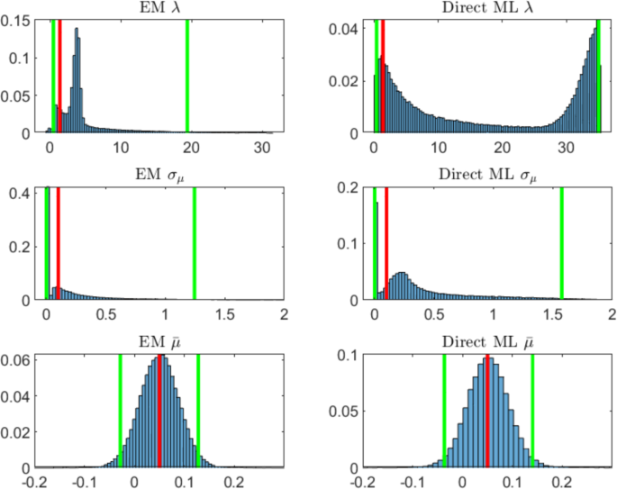
Probability histograms of parameters estimated via EM algorithm (left panels) and via direct likelihood maximization of innovation process (right panels) for years of daily observations and 100,000 simulations. The red line indicates the true value of the parameter, the green lines the 2.5% and 97.5% quantiles. The simulation parameters set is (color figure online)
For and years (Table 1, Panel B), we observe a positive effect on the estimates due to the longer time series at our disposal. Indeed the width of the quantile intervals is approximately halved with respect to the estimates with 10 years data. Figure 2 shows the histograms of the estimations of the parameters in this case. The estimated distributions are still not satisfactory except for . The mean over the simulated paths of the estimated volatility of the observed process is .
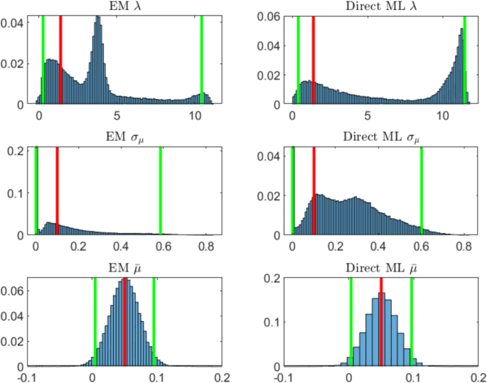
Probability histograms of parameters estimated via EM algorithm (left panels) and via direct likelihood maximization of innovation process (right panels) for years of daily observations and 100,000 simulations. The red line indicates the true value of the parameter, the green lines the 2.5% and 97.5% quantiles. The simulation parameters set is
For and years (Table 1, Panel C), the estimates for the parameter and improve on average and their quantile intervals are a little stricter than the ones obtained in the previous case. On the other hand, the estimates of have larger quantile intervals. This is due to the fact that while a higher value of makes the drift more visible from one hand, from the other hand it also makes the drift process more volatile. Hence, it is more difficult to estimate the long-term mean because the fluctuations of the latent process are very wide. Figure 3 shows the estimated distributions of the parameters obtained by the two procedures. Now the two estimation methods provide approximately the same distributions. This is due to the fact that, when the latent process is visible, most of the fluctuations of the observed process come from the latent process. The mean over the simulated paths of the estimated volatility of the observed process is .
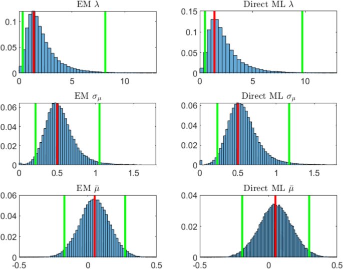
Probability histograms of parameters estimated via EM algorithm (left panels) and via direct likelihood maximization of innovation process (right panels) for years of daily observations and 100,000 simulations. The red line indicates the true value of the parameter, the green lines the 2.5% and 97.5% quantiles. The simulation parameters set is
For and years (Table 1, Panel D), it is tangible the combined effect of the high weight of the latent process with respect to the observed process, and the size of data given by the longer time series. In this case we obtain the best estimates on average and the strictest quantile intervals. Figure 4 shows the estimated distributions of the parameters. The mean over the simulated paths of the estimated volatility of the observed process is .
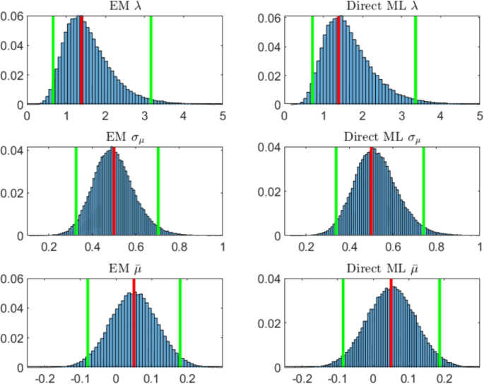
Probability histograms of parameters estimated via EM algorithm (left panels) and via direct likelihood maximization of innovation process (right panels) for years of daily observations and 100,000 simulations. The red line indicates the true value of the parameter, the green lines the 2.5% and 97.5% quantiles. The simulation parameters set is (color figure online)
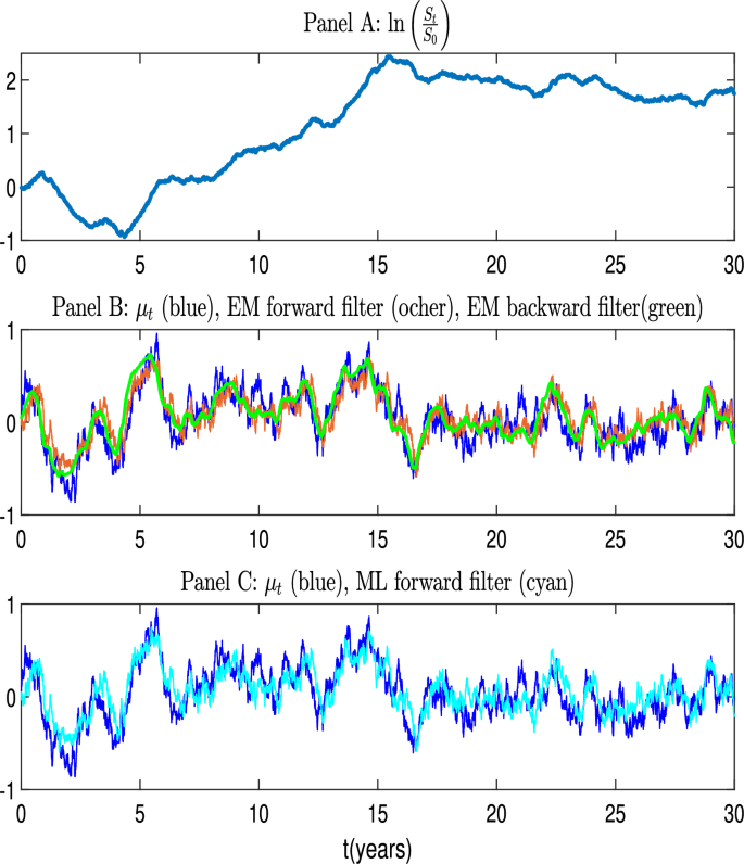
Example of a simulated path with good estimation properties. The figure shows the cumulative log-return (Panel A), the latent process compared to the forward and backward filters, evaluated with the parameters estimated via the EM algorithm (Panel B), and to the forward filter evaluated with the parameter estimated by the direct likelihood maximization of the innovation process (Panel C). True model parameters are as in Table 1, Panel D. EM estimations: , . Direct likelihood maximization estimations:
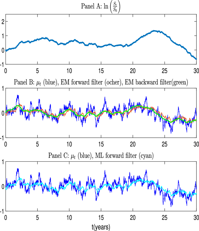
Example of a simulated path with poor estimation properties. The figure shows the cumulative log-return (Panel A), the latent process compared to the forward and backward filters, evaluated with the parameters estimated via the EM algorithm (Panel B), and to the forward filter evaluated with the parameter estimated by the direct likelihood maximization of the innovation process (Panel C). True model parameters are as in Table 1, Panel D. EM estimations: . Direct likelihood maximization estimations:
We conclude the numerical illustration by selecting two particular paths among those generated for and years, to show how path realization may influence the performance of estimations. It may happen indeed that the estimates are not accurate even though is high and the available time series is long. In what follows we present one case in which the estimates are accurate and one case in which they are not. Figure 5 shows a favorable path realization providing good parameter estimates while Fig. 6 shows the case with poor parameter estimates. Panel A of each figure shows the realized path of the cumulative log-return . The simulated path of the latent process is compared to the forward and backward filters, evaluated with the parameters estimated via the EM algorithm (Panel B), and to the forward filter evaluated with the parameters estimated by the direct likelihood maximization of the innovation process (Panel C)Footnote1.
In Fig. 5 we can see that the filters provide an accurate representation of the latent process, except for a few peaks. In this case the estimates are close to the true ones. More specifically, the parameters estimated by the EM algorithm are , and . The estimations through the direct likelihood maximization over the realized innovation process are , and .
Figure 6 shows the case when the filters fail to catch the fluctuations of the latent process and the estimates are far from the true values. The EM estimates are . The parameters estimated with the other method are .
The main difference between the two paths of the latent process shown above lies in the presence of more pronounced peaks in the unfavorable scenario depicted in Fig. 6 that the filter has no time to capture properly. Conversely, in the favorable scenario of Fig. 5, the peaks are fewer in number, less pronounced, and occur more gradually.
4.2 Parameter misspecification: the impact on trading strategies
To investigate the potential limitations of the estimation process and their implications for practical applications, we analyze the impact of misspecifying the speed of mean reversion, , on trading strategies. We anchor our discussion by considering the framework developed by Garleanu and Pedersen (2013). In their setup, the objective is to derive an optimal investment strategy that maximizes the expected risk-adjusted returns, accounting for transaction costs. They analyze a setting with discrete trading times, where asset returns are linearly dependent on a set of risk drivers that follow mean-reverting dynamics. In our case we have just one asset depending on one risk driver, the drift parameter.
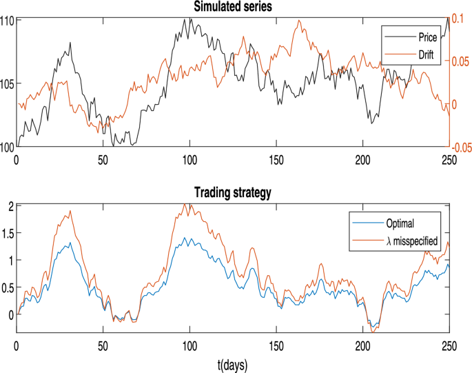
Trading under Misspecification of the Speed of Mean Reversion. The upper panel displays a daily time series of the price (left vertical axis) and drift parameters (right vertical axis). The lower panel illustrates the optimal policy, as computed using Eq. (4.1), alongside the policy derived under a misspecified value of the speed of mean reversion. Parameters are as follows: , , corresponding to a half-life of 6 months, the misspecified value is corresponding to a half-life of 1 year and half. The other parameters are set as and
In Example 1, Equation (22) of Garleanu and Pedersen (2013), the authors provide the optimal policy at time t as a function of the parameters of the model when trading just a single asset. For the convenience of the reader, we reproduce this expression here, using our notation and assuming that the long-term mean of is zero:
where
and where is the risk aversion parameter, transaction costs are quadratic in changes of the position and proportional to , c is the proportionality constant for transaction costs, the interest rate used to discount the future cash flows is and
From Eq. (4.1), we observe that the optimal position at time t is a linear combination of the previous position and the term . The component is particularly important, as it accounts for the expectation of all future positions based on the current signal. When transaction costs are high (i.e. a large c), the weight on decreases, which naturally slows down trading, as the costs discourage frequent adjustments to the position.
An insightful feature of Eq. (4.1) is its indication of how the optimal policy varies with the persistence of the signal, as measured by the speed of mean reversion . For a highly persistent signal (i.e. a lower ), the impact of on the policy is stronger than that of the current position , reflecting the expectation that the signal will remain stable over time. Conversely, if the signal mean-reverts quickly (a high ), the portfolio manager gives greater emphasis to the current position, as the signal is expected to change rapidly, making it less advantageous to lean toward the longer-term target.
When misestimating , we find distinct effects on trading intensity. Overestimating leads the manager to assume the signal is less persistent than it actually is, causing them to reduce trading frequency relative to the optimal policy. The perceived transience of the signal results in a stronger preference to remain close to the current position rather than adjusting toward . Underestimating has the opposite effect: it causes the manager to view the signal as more persistent than it truly is, leading to an increase in trading intensity. The manager trades more aggressively toward , as she/he incorrectly believes that the signal will endure longer, making it worthwhile to invest in alignment with it.
Thus, misestimating can lead to substantial deviations from the optimal trading strategy, either by dampening the response to genuine opportunities or by increasing trading costs due to excessive rebalancing. This underscores the critical importance of accurate calibration of for effective trading strategy implementation.
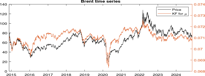
Time series of the price of Brent Oil (Ticker: ’BZ = F’) (left vertical axis) alongside the estimated latent drift obtained from the Kalman filter (right vertical axis). Parameter estimates are , , and
As an example, Fig. 7 presents a simulated path of the price (left vertical axis) and the drift parameter (right vertical axis) over a 1-year period (upper panel). The lower panel illustrates the optimal trading strategy, superimposed with a strategy derived under a misspecified value of the speed of mean reversion. In this example we set , and , corresponding to a half-life of 6 months. The optimal policy is computed by using the correct value of in the denominator of Eq. (4.1), while the Kalman filter for the drift is employed to obtain the best estimate of . In contrast, the suboptimal strategy is derived using the same filter for but a misspecified value of in (4.1). Specifically, the misspecified value is corresponding to a half-life of 1 year and half. The other parameters are set as and .
As anticipated, underestimating the speed of mean reversion causes the trader to deviate from the optimal policy by increasing the intensity of trading. This occurs because the trader believes the signal is more persistent than it actually is.
4.3 Estimation on a real time-series
Here, we test the model using real-world data. Specifically, we analyze the time series of Brent Oil prices (Ticker: BZ = F) over a 10-year period from November 2014 to November 2024. The model is estimated using the EM algorithm, yielding the following parameter estimates: , , and . Figure 8 displays the time series of prices alongside the Kalman Filter estimate of the latent drift process (shown on the right axis).
The estimated volatility of the drift process is significantly smaller than . This implies that the majority of the variance in the price process originates from the innovation term, rather than from the drift component. Consequently, the latent drift provides a relatively stable, long-term trend, while short-term price movements are predominantly driven by high-frequency shocks and noise. As argued in Sect. 4.1, in such a scenario, the latent drift becomes challenging to detect directly, as it is overshadowed by the much larger volatility of the innovation term. However, with real market data, the realization of the latent factor is unknown, making it impossible to distinguish between a misspecified model and a properly specified model with misestimated parameters. In the former case, the high innovation variance arises because the model fails to adequately represent the observed data, whereas in the latter case, it is a consequence of inaccuracies in parameter estimation.
5 Conclusions
We considered a stock price process driven by a latent drift which is mean-reverting. Our investigation focused on assessing the accuracy of parameter estimation for this latent process across a large set of simulated paths. We employed two distinct maximum likelihood-based methods: the EM algorithm and direct maximization of the likelihood of innovations. This modeling approach is commonly utilized in financial literature for asset allocation under partial information.
The ratio of the volatility of the latent process to that of the observed process plays a critical role in the estimation procedure’s effectiveness. Higher volatility ratios enable filters to better track the latent process, yielding estimates closer to true values. Conversely, lower volatility ratios lead to filter inefficacy in detecting the latent process, resulting in poor estimation performance. Surprisingly, our numerical analysis reveals that even with high volatility ratios, filtering struggles to accurately estimate the latent process. Performance notably improves when learning about the latent process is informed by 30 years of daily data. Nonetheless, substantial deviations from simulated parameters persist in many path realizations, challenging the widely accepted model’s efficacy. We offer an explanation for this discrepancy through a simple dimensional analysis, which highlights the scaling effect of the latent process’s weight in the observable data. This scaling underscores the necessity for a large volume of observations to glean meaningful insights into the latent process.
This analysis highlights several open questions for future research. Given that the model proposed is widely used in the literature on quantitative financial management due to its analytical tractability and interpretability, the key issue that arises is how to improve the precision of the estimates. One potential approach is to estimate the model by integrating the stochastic differential equations that describe its dynamics and then sampling the data at observation times, rather than relying on Euler discretization for practical implementation. This adjustment could be beneficial, as the issue appears to be related to the scaling properties of the model parameters. Furthermore, improving optimization through robust algorithms, which explore the parameter space more thoroughly in search of a global maximum, or by using better initialization, could enhance the likelihood maximization of the innovations. However, this may not be effective in the EM approach, as the maximization step is solved analytically in this context. An alternative approach worth exploring is the use of other filtering techniques, such as particle filters, which are well-suited for dealing with latent variables and could potentially provide more reliable estimates of the latent factors.