Article Content
1 Introduction
1.1 Background
Mechanical mechanisms are developed to fulfill specific tasks, yet it is often possible to use multiple types of mechanisms to achieve the same overall function (McGovern and Sandor 1973; Xu and Liu 2024). In industrial applications, vehicle suspension systems serve as a prime example of this versatility in mechanical design (Jiregna and Sirata 2020). The primary objective of a vehicle suspension system is to enhance ride quality and handling by isolating the vehicle body from road irregularities and maintaining stable contact with the road surface. To accomplish this, various suspension configurations are utilized, including MacPherson struts, double wishbone, and multi-link systems, each with its own distinct structure, performance characteristics, and application suitability. For example, MacPherson struts are commonly used for their simplicity and cost-effectiveness, whereas double wishbone suspensions are favored in performance-oriented vehicles for their superior control over wheel alignment. Multi-link systems, on the other hand, offer flexibility in design adjustments, making them ideal for premium vehicles where ride quality and handling are both priorities (Jiregna and Sirata 2020; Sharp and Crolla 1987). The process of selecting a suitable suspension type is inherently complex because each configuration presents a unique balance of advantages and limitations, which vary based on factors like vehicle type, intended usage, and cost constraints. Consequently, choosing the optimal suspension system requires a thorough evaluation of these trade-offs to meet specific performance and comfort requirements. This complexity underlines the need for advanced design and optimization methods to support engineers in making informed decisions in suspension mechanism selection, which is a key focus of the proposed multi-fidelity framework in this study.
Meta-heuristic algorithms, inspired by natural and biological processes, are optimization methods used to solve complex problems without requiring derivative information. Recently, these algorithms have shown effectiveness in optimizing large-scale mechanical structures, such as bridges, dams, and similar structures, requiring precise condition assessments and reliability analyses (Qin et al. 2024; Li et al. 2024; Tran et al. 2023). Methods like the Artificial Fish Swarm Algorithm (AFSA) and Termite Life Cycle Optimizer (TLCO) have proven beneficial in optimizing structural integrity and efficiency in civil engineering applications, demonstrating high computational efficiency for large-scale problems. Although primarily developed for civil engineering, these approaches have potential application in other fields, with adaptation possible for similarly complex systems like vehicle suspension design.
In particular, studies on vibration and buckling optimization for functionally graded structures using advanced hybrid methods, such as combining artificial neural networks (ANNs) with meta-heuristic techniques, have revealed significant improvements in both computational efficiency and predictive accuracy (Tran et al. 2023; Bai et al. 2024). These methods highlight the potential benefits of combining machine learning and optimization in scenarios with high computational demands and complex structural behavior, making them promising tools for applications beyond their original scope. Similarly, integrating deep neural networks (DNNs) with evolved optimization algorithms has yielded promising results in damage detection for intricate structures like truss bridges (Nguyen-Ngoc et al. 2024). While these approaches offer robustness and precision in handling large datasets from structural health monitoring, they also exhibit limitations, such as high computational costs and sensitivity to model parameter tuning. Addressing these limitations is crucial for future research, especially as applications extend to similarly demanding fields.
Recently, the automotive industry has increasingly relied on computational methods to enhance suspension design processes (Koulocheris et al. 2017; Reddy et al. 2016; Fujita et al. 1998). Traditional design approaches have typically involved sampling specific design solutions within the design space, performing analyses on these discrete samples, and then progressing to more detailed designs based on the most promising samples. However, this method has a significant drawback: it only evaluates the potential of a given design space through its discrete samples, thus failing to fully exploit the potential within the entire design space. With the advent of artificial intelligence, researchers sought to overcome these limitations by using predictive models such as deep learning to select optimal values from continuous design variables (Kim et al. 2022; Panchal et al. 2019; Patel et al. 2021; Ramu et al. 2022). This innovation aimed to streamline the design process and maximize the potential of the design space. Nonetheless, as product development progresses, the analysis environment typically transitions from low- to high-fidelity simulations, reducing the number of samples available for high-fidelity analysis. Despite constructing a robust learning model using low-fidelity analysis data, there is still uncertainty about performance metrics in high-fidelity analyses due to potential discrepancies between low-fidelity and high-fidelity results. For example, assumptions applied in the low-fidelity analysis (e.g., rigid body analysis, ignoring friction) could yield different performance metrics under the same conditions in the high-fidelity analysis. Such differences, if considerable, can lead to critical issues that cannot be ignored. In addition, selecting the most appropriate suspension type and design parameters remains challenging, given the need to balance multiple objectives, such as minimizing suspension travel, acceleration and maximizing durability.
These challenges are encountered in real-world design scenarios, where the iterative process often has multiple stages and is sensitive to changes in target values due to shifting design criteria or insights gained from intermediate analysis results. Thus, any changes in target specifications require recalculations and potentially additional simulations, substantially increasing the computational cost. When combined with performance discrepancies that may arise from transitioning between different fidelity levels, these design scenarios can lead to exponentially increasing costs and time requirements during iterative design cycles(Wynn and Eckert 2017).
1.2 Research goal
In this paper, to effectively improve the mentioned challenges, we propose a multi-fidelity design framework aimed at recommending optimal types and designs of mechanical mechanisms, specifically vehicle suspension systems. Our approach integrates low-fidelity (rigid body dynamics) analyses with high-fidelity (multi-flexible body dynamics) simulations, using deep learning-based surrogate models to bridge the gap between fidelity levels. The multi-fidelity approach balances computational efficiency and prediction performance metrics by combining low-fidelity, cost-effective simulations with high-fidelity, accurate simulations. This ensures that the potential within the design space is significantly utilized and that the limitations of both traditional and AI-based design methods are significantly improved. Using advanced data mining techniques and multi-objective optimization, we aim to provide designers with robust guidelines and optimized solutions for suspension design.
In vehicle suspensions, specific performance metrics can be optimized for minimization or maximization, such as minimizing suspension travel, acceleration, or maximizing durability. However, some performance metrics, such as first-mode frequency, cannot simply be optimized for higher or lower values but must be considered to satisfy detailed design specifications. Target values may change depending on the purpose or desired performance of the vehicle, making it difficult to achieve a single optimal solution during the design process. Therefore, recommending the optimal type and design variables corresponding to frequently shifting target values can be an effective approach to maximizing the potential of the design space. This distinction is critical to achieving balanced and effective suspension designs. In particular, our framework enables designers to input the sprung mass of a vehicle and generate optimal design solutions for several suspension types based on different first-mode frequencies. Designers can select the most appropriate design configuration from these Pareto optimal solutions. We will demonstrate the effectiveness of our framework through a case study on three types of suspensions, including MacPherson strut and double wishbone (low & high mount) suspensions. The results will demonstrate the potential of our approach to increase design efficiency, reduce costs, and improve overall vehicle performance. The main contributions of this framework can be summarized as follows:
- 1.To the best of our knowledge, this is the first study to propose an integrated multi-fidelity framework that combines traditional engineering principles with AI-driven deep learning models for vehicle suspension mechanism optimization. This framework uniquely merges low-fidelity rigid body dynamic analysis with high-fidelity flexible body dynamic analysis, enabling scalable and continuous performance predictions that address the limitations of traditional discrete sample evaluations.
- 2.The framework enables effective multi-objective optimization across multiple suspension types, including MacPherson strut and double wishbone (low & high mount) configurations. This approach facilitates the generation of Pareto optimal design solutions that align with various target first-mode frequencies, allowing designers to select the most suitable suspension configuration for specific vehicle performance requirements.
- 3.Provide practical design guidelines by extracting fundamental design rules from Pareto solutions using data mining techniques, aiding in the future design of vehicle suspension systems.
- 4.The proposed methodology is validated through a comprehensive case study on three types of suspension systems, showcasing its potential to enhance design efficiency, reduce costs, and improve overall vehicle performance.
This paper is organized as follows. Section 2 summarizes the related studies, and Sect. 3 covers the overall framework introduction and methodology for each stage. Section 4 includes discussions by extracting the application results and design rules of the proposed framework, and compares the proposed framework with the conventional AI-based approach applied to suspension design. Finally, Sect. 5 includes conclusions, limitations, and future work.
2 Related works
In recent years, the industrial field has increasingly turned to artificial intelligence (AI) models, particularly deep learning, to address complex engineering challenges. Deep learning models can effectively utilize vast amounts of data continuously accumulated in the industry(Ullman et al. 1988; Krahe et al. 2022; Shan and Wang 2010), such as automotive systems(Kang et al. 2014; Shin et al. 2023; Grigorescu et al. 2020; Gobbi and Mastinu 2001; Alkhatib et al. 2004; Abdelkareem et al. 2018), automated robotic manipulators(Wang et al. 2020; Purwar and Chakraborty 2023; Soori et al. 2023), smart factories (Chen et al. 2017; Kotsiopoulos et al. 2021), and beyond (Panchal et al. 2019; Patel et al. 2021). Specifically, it has the potential to significantly enhance computational efficiency and accuracy in processes that traditionally rely on resource-intensive simulations like finite element analysis (FEA) and computational fluid dynamics (CFD) (Zhao et al. 2021; Phiboon et al. 2021; Kennedy and O’Hagan 2000). The trend toward AI-driven solutions has led to various studies of optimization or methodologies to take advantage of the engineering field. One noted field of research within this broader trend is the application of deep learning techniques to the design and optimization of mechanical mechanisms. Xue et al. (2023) explored a data-driven approach that maximizes computational efficiency by offering complex dynamic analysis solutions, extending the application of deep learning-based solvers to predict smooth solutions. This advancement is particularly crucial in scenarios where traditional methods struggle with the computational demands of real-time or high-fidelity simulations. Additionally, Go et al. (2024) introduced an efficient method combining deep learning models with principal component analysis (PCA). This method leverages PCA to reduce the dimension of large datasets, enabling faster training times without compromising accuracy. Chen et al. (2015) conducted a study using kriging surrogate models for multi-objective optimization to improve vehicle ride comfort. This study bears similarities to the multi-objective optimization methods discussed in this paper, particularly in its goal of elucidating the relationship between design parameters and ride comfort. However, our proposed method differs by addressing scenarios where design decisions must be based solely on reference performance and simultaneously considering various suspension mechanism types. This distinction allows for a broader design space exploration, thereby enhancing the potential to obtain optimal performance.
Despite these advances, the conventional product design process typically involves multiple stages or iterations, each requiring different analysis conditions(Yoo et al. 2021; Lei et al. 2022; Schlicht et al. 2021). The early stages of the design process often focus on prototype exploration, emphasizing simplified modeling and functionality. In contrast, later stages involve conducting high-fidelity simulations (such as FEA or CFD) on designs derived from earlier explorations to optimize and reduce the candidate design space. However, this traditional approach is not without its limitations. First, there is a significant mismatch between the analysis environments and the types of performance metrics considered at each stage. For example, rigid body dynamics analysis does not account for deformation, making it impossible to calculate maximum stress values. On the other hand, transient dynamics analysis partially incorporates finite element methods, allowing for the calculation of maximum stress. This fundamental difference underscores the challenge of aligning performance metrics across different stages of the design process. Second, as the process progresses to stages requiring high-fidelity simulations, the number of explored designs and candidate solutions tends to decrease exponentially. This presents a significant challenge, particularly given the limited availability of sufficient datasets for the effective application of deep learning methods. In order to address the issues of data scarcity and high computational costs prevalent in the high-fidelity simulation stages, the concept of multi-fidelity has been proposed(Forrester et al. 2007; Han and Görtz 2012; Peherstorfer et al. 2018). The multi-fidelity approach aims to balance the accuracy of models derived from low- and high-fidelity simulations, providing a more efficient framework for optimization across various stages of the design process.
Multi-fidelity models have also been found to be applicable in flexible multibody dynamics analysis, where they address the computational challenges posed by including nonlinearities in dynamic simulations. Han et al. (2021) proposed an algorithm for efficiently training a two-stage deep neural network designed for dynamic simulations that require nonlinear considerations. This approach targets the substantial computational costs of transient dynamic analysis including flexible bodies. Additionally, Xue et al. (2023) utilized analytical models of suspension systems and multibody models as low- and high-fidelity models to solve optimization problems related to filtering vibrations from road surfaces. While this approach is well-suited for guiding exploration during the early stages of the design process, it is essential to note that simplified models may not fully capture the complex nonlinear geometries inherent in multiple mechanisms.
Most cases mentioned above focus on optimization problems within the design process. However, in real-world design process scenarios, there are instances where design decisions must be referenced by performance values that cannot be optimized (Gomes 2016; Beck et al. 1999; Privitera et al. 2017; Xu et al. 2022; Zhang et al. 2023; Xie et al. 2013). The main application proposed for vehicle suspension in this paper is that the natural frequency of a vehicle suspension system must be selected based on the vehicle’s intended use and driving conditions, ensuring it remains within a specific range. Various factors, such as the joint position in the mechanism, sprung mass, and the mechanical properties of the shock absorber, influence the natural frequency of a suspension system. However, discrepancies in natural frequency values can arise between low-fidelity analyses (rigid body dynamics) and high-fidelity analyses (transient dynamics), underscoring the need for a multi-fidelity framework. Moreover, the optimal design solutions corresponding to the selected natural frequency may differ, necessitating real-time analysis and recommendation of optimal design distributions for the specified frequency. This study addresses the challenge of optimizing design solutions while improving data scarcity and performance inconsistency between high- and low-fidelity simulations.
3 Multi-fidelity suspension design optimization framework
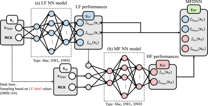
The deep learning-based multi-fidelity mechanism design framework proposed in this study consists of five stages, and its overall flowchart is shown in Fig. 1. First of all, three types of suspensions are defined, and they are sampled by the functions that calculate the joints of the parametric-based mechanisms (Stage 1). Then, the design sample in the design space is converted into a 3D CAD model through parametric design (Stage 2). Based on the joint and geometric conditions calculated in Stage 1, an assembling for automatic dynamic analysis is established and used for low-fidelity and high-fidelity analysis (Stage 3). To predict the performance metrics of each suspension type, we train a multi-fidelity model based on the data performed in the low-fidelity and high-fidelity analysis (Stage 4). Finally, the already trained multi-fidelity surrogate model recommends optimal types and parameters via the non-dominated sorting genetic algorithm-II (NSGA-II) (Stage 5). The following subsections are organized to detail each stage of the proposed framework.
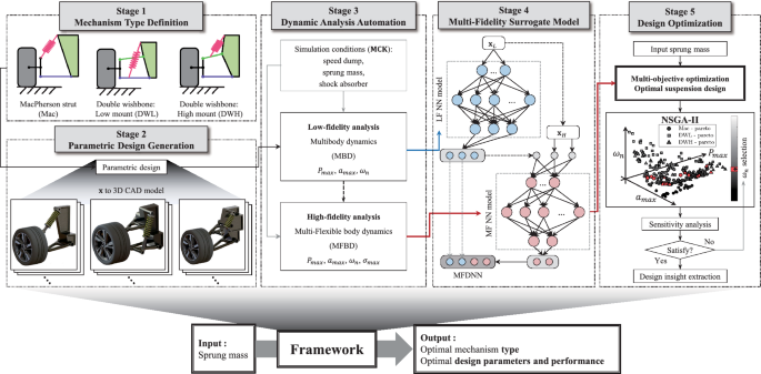
Multi-fidelity suspension design optimization framework
3.1 Stage 1: Mechanism type definition
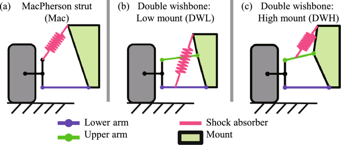
In Stage 1, several mechanism types of the suspension system selected for the proposed application of the framework are defined. A suspension system’s primary function is to mitigate vibrations experienced during road driving, thereby enhancing vehicle stability and ride comfort. Consequently, the suspension must provide degrees of freedom between the wheel and the vehicle body, with shock absorbers to effectively absorb vibrations. Suspension systems enable relative motion between the wheel and the vehicle body while damping vibrations. This is primarily achieved through springs and shock absorbers, with the configuration varying depending on the type of suspension mechanism. This study focuses on three representative types of suspension systems as shown in Fig. 2: MacPherson strut, double wishbone (low mount), and double wishbone (high mount). The descriptions of each type and geometrical condition are as follows:
Suspension mechanism type definition
3.1.1 Type 1: MacPherson strut suspension
The MacPherson strut(in Fig. 2 (a)) is one of the simplest forms of suspension systems, commonly used for front wheels. Its design is advantageous due to the reduced number of components and a relatively straightforward structure, making it easy to manufacture and cost-effective. The MacPherson strut comprises a single strut (integrating the spring and shock absorber) and a lower control arm, offering benefits in space savings and weight reduction. However, it provides relatively low lateral rigidity, making it less suitable for high-performance vehicles.
For the MacPherson strut type, four design parameters are shown in Fig. 3. Three of them are independent variables, and one is a dependent variable based on the calculation of the independent variables. is the length of the lower arm. , which has a value between 0 and 1 to prevent infeasible mechanism generation, calculates the x position where the shock absorber is fixed to the mount by multiplying . is the mounting height between the shock absorber and the lower arm. , the length of the shock absorber, is derived from the geometric relationship between , , and , making it a dependent variable calculated from the other parameters. The equation for calculating the length of is provided in Eq. (1).
where is the constant knuckle height.
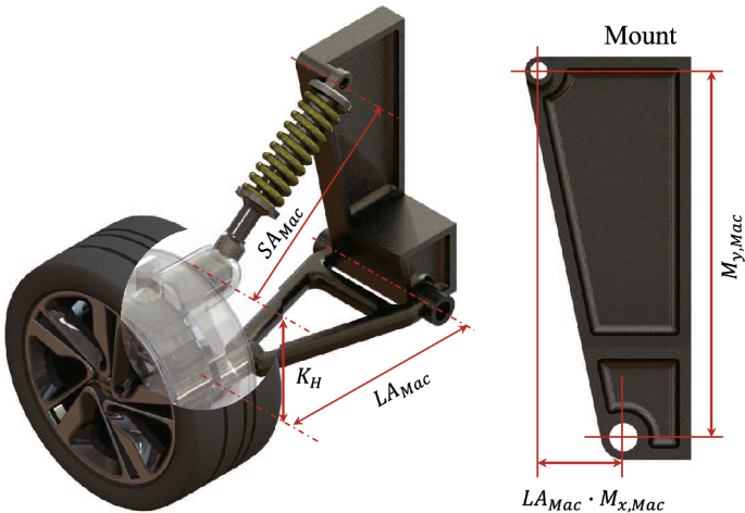
MacPherson strut suspension design parameter and 3D configuration
3.1.2 Type 2: Double wishbone suspension (low mount)
The double wishbone suspension(in Fig. 2 (b)) consists of two A-shaped control arms (upper and lower arms), allowing for more precise control of wheel movement. In the low mount type, the shock absorber is attached to the lower arm, providing a lower center of gravity and stable steering characteristics. Despite the complexity and higher manufacturing cost, the double wishbone suspension offers superior handling and ride comfort, making it ideal for high-performance vehicles.
For the Double wishbone (low mount) type, there are eight design parameters(in Fig. 4): six independent variables and two dependent variables. is the length of the lower arm. , a ratio value, calculates the x position where the shock absorber is fixed by multiplying it with . , a ratio value to calculate the x position where the upper arm is fixed to the mount, calculated by multiplying . is the ratio value to calculate the y position where the upper arm is fixed to the mount, calculated by multiplying . is the ratio for calculating the x position where the shock absorber is fixed to the mount, calculated by multiplying the ratio with . represents the total height of the mount.
and , the lengths of the upper arm and the shock absorber, respectively, are dependent variables derived from the geometric relationships between the six independent variables. The equations for determining the lengths of and are provided in Eq. (2) and (3).
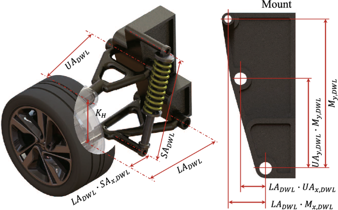
Double Wishbone (low mount) suspension design parameter and 3D configuration
3.1.3 Type 3: Double wishbone suspension (high mount)
The high mount type of double wishbone suspension (in Fig. 2(c)) features the shock absorber attached to the upper arm. This configuration extends the range of motion for the suspension and enhances performance across various driving conditions. High mount suspensions are predominantly used in racing cars or high-performance sports cars, where maximizing stability during high-speed driving is crucial.
Although The low mount type of double wishbone (DWL) and high mount type of double wishbone (DWH) configurations may appear to share the same number and range of design variables, they are fundamentally different mechanisms with distinct design objectives. Specifically, the DWH configuration has the shock absorber attached to the upper arm, while the DWL configuration attaches the shock absorber to the lower arm. This variation impacts the suspension’s kinematic behavior, making the two types suited to different performance requirements. For example, the DWH is often utilized in high-performance or racing vehicles, where enhanced stability and a wider range of motion are critical under high-speed conditions.
To simplify the suspension mechanism design problem and focus on generalizable design scenarios, the design variables chosen in this study reflect a somewhat simplified or controlled set. While similar ranges indeed constrain them, each variable is selected to accurately represent the distinct kinematic characteristics and mechanical constraints of each suspension type. This intentional selection ensures that the proposed framework remains flexible yet realistic for different suspension mechanisms despite some overlap in variable definitions.
For the Double Wishbone (high mount) type, there are eight design parameters (in Fig. 5): six independent variables and two dependent variables. is the length of the lower arm. , a ratio value, calculates the x position where the shock absorber is fixed by multiplying it with . , a ratio value to calculate the x position where the upper arm is fixed to the mount, is calculated by multiplying . is the ratio value to calculate the y position where the upper arm is fixed to the mount, calculated by multiplying . is the ratio for calculating the x position where the shock absorber is fixed to the mount, calculated by multiplying the ratio with . represents the total height of the mount.
and , the lengths of the upper arm and the shock absorber, respectively, are dependent variables derived from the geometric relationships between the six independent variables. The equations for determining the lengths of and are provided in Eq. (4) to (9).
To calculate the length of the shock absorber, it is first necessary to calculate the x and y positions that have been fixed to the upper arm. These positions can be calculated by combining the declared design parameters, and the process is as follows:
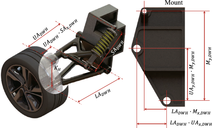
Double wishbone (high mount) suspension design parameter and 3D configuration
3.2 Stage 2: Parametric design generation
To generate design variables for each suspension type, the Latin Hypercube Sampling (LHS) technique was employed. LHS is a statistical method that evenly samples the design space, ensuring that the possible values of each variable are uniformly distributed. This approach allows for a wide range of design variable combinations, facilitating the exploration of numerous design possibilities. Once the design variables were generated using LHS, these variables were utilized to automatically create 3D CAD models. For this purpose, Rhinoceros 3D software was used (McNeel et al. 2020). Rhino Grasshopper is a powerful parametric design tool that enables the automatic generation of 3D models based on input variables. As mentioned in Stage 1, each type of suspension design parameter description and sampling range is shown in Table 1.
In practical research scenarios, it is often not feasible to utilize the entirety of available computational resources or sample spaces, and hence, a strategic reduction in sample size is necessary. In this study, although the optimal conditions suggest an extensive dataset for solving the optimization problems effectively, we pragmatically constrained our samples to a manageable number for computational efficiency and practical feasibility. Specifically, for the suspension system problem at hand, we have deliberately chosen to limit the number of samples to ensure a balance between computational efficiency and the quality of the optimization results.
To generate suspension design samples using LHS(Table 1), approximately 500 samples were initially created for each type. However, when design variables are sampled independently, it is common for certain configurations to be infeasible within specific ranges, particularly in mechanism-dependent designs where variables are geometrically interdependent. Therefore, after applying constraints specific to each suspension type to ensure feasible configurations, a filtered set of samples was retained. For the MacPherson strut suspension type, 300 samples were generated; for the double wishbone low mount type, 209 samples were used; and for the double wishbone high mount type, 200 samples were selected. This strategic selection of sample sizes was made to maintain a reasonable computational burden while still providing a robust exploration of the design space. By choosing these specific sample sizes, we ensure that the optimization process remains efficient and manageable, reflecting a pragmatic approach in real-world applications.
3.3 Stage 3: Dynamic analysis automation
In Stage 3, the objective is to analyze the dynamic behavior of each suspension system, which has been converted into a 3D CAD model. The data obtained from these analyses will be employed as labels for surrogate model training in Stage 4.
The suspensions generated in Stage 1 and 2 were randomly selected within a limited LHS range, consequently lacking insight into their physical performance. For relatively simple mechanisms like the MacPherson strut suspension, an exact solution can be derived using the governing equations of a 2-mass system. However, in the case of actual suspensions, the assumptions required to formulate differential equations are more complex. Additionally, for double wishbone suspensions, the nonlinear displacements resulting from the mechanical structure suggest that solving the problem using governing equations is inherently limited. Therefore, to achieve an optimal mechanism that considers performance, design optimization through a surrogate model is a more effective approach.
3.3.1 Dynamic analysis setup
In the dynamic analysis, the mount sprung mass () and the shock absorber’s damping coefficient () and stiffness () were varied. The MCK parameters mentioned above were then input into the dynamic simulation software RecurDyn 2023.
Conventionally, vehicle suspension design relies on standardized shock absorbers with fixed mechanical properties, which limits the flexibility and potential scope of the design space. To enhance the potential design space and provide a more adaptable and generalized framework, this study treats the shock absorber properties (stiffness and damping coefficient ) and mount mass () as variable design parameters rather than fixed values. The range of values for these parameters was sampled using the Latin Hypercube Sampling (LHS) method to generate 50 diverse combinations (Table 2). This sampling approach strikes a balance between adequately exploring the design space and managing computational efficiency, given that each suspension mechanism must undergo dynamic analysis under all 50 parameter sets. Thus, the 50 LHS samples were selected to maximize design flexibility within computational limits, allowing the framework to generalize to a broader array of suspension configurations while maintaining manageable simulation costs.
For the tire, stiffness () and damping coefficients () were also specified to approximate typical ranges observed in passenger vehicles. Literature reports common values for tire stiffness within the range of 150 to 300 and damping coefficients between 1.5 and 3 , as established in multiple studies on tire behavior under dynamic loads (Pacejka 2005; Godbole et al. 2021; Yang et al. 2019). The current study selected for stiffness and for damping as representative values for standard conditions (Fig. 6), balancing typical performance metrics and computational stability. These settings provide a basis for assessing suspension response within the scope of the analysis’s intended application and simulation constraints.
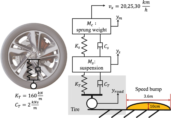
Tire and road condition configuration
To predict the performance metrics of the sprung mass () and the shock absorber () for each suspension model, dynamic analyses were conducted under various conditions. The dynamic analysis assumes the vehicle drives over a typical speed bump at 20, 25, and 30km/h. The speed bump used in the analysis has a convex shape with a width of 3.6m and a 10cm height, representing common dimensions found in real-world environments(in Fig. 6). This profile was applied to the ground in the dynamic simulations to ensure realistic testing conditions. These conditions were used to simulate real-world driving scenarios and to evaluate the performance of the suspensions under different speeds (Godbole et al. 2021; Xiao et al. 2020).
3.3.2 Low-fidelity analysis: multibody dynamics(MBD)
This study distinguishes between low-fidelity and high-fidelity analyses to establish a multi-fidelity approach. In this section, we perform a low-fidelity analysis using Multibody Dynamics (MBD) to evaluate the suspension systems under various conditions. This analysis uses rigid body dynamics, where each part of the suspension is assumed to be a rigid body. The dynamic response of each suspension mechanism as it travels over a speed bump is analyzed to extract three performance metrics(in Fig. 7 (a)):
Maximum suspension travel (): This metric measures the maximum relative vertical displacement of the mount, excluding any bias from the initial vehicle height. It is determined by calculating the difference between the maximum and minimum vertical positions of the mount as the vehicle passes over the speed bump. This provides insight into the suspension’s ability to absorb shocks and maintain vehicle stability.
Maximum acceleration (): This metric captures the peak acceleration experienced by the mount. It is crucial for assessing the ride comfort and the impact of sudden shocks on the vehicle’s structure and passengers. During road driving, the variability in surface conditions, such as uneven pavement or speed bumps, can cause significant changes in due to inertial effects. Such irregularities in the road surface play an essential role in influencing sudden impacts and ride quality, as they contribute to the transient forces experienced by the suspension system, affecting passenger comfort and vehicle stability.
First-mode natural frequency (): In addition to the other metrics, we conduct an eigenvalue analysis to determine the natural frequencies of the suspension systems. Our specific focus is on the first mode of vibration, which provides a deep understanding of the system’s inherent dynamic behavior. This frequency serves as a reference for understanding the system’s resonance characteristics and potential susceptibility to vibration issues.
By analyzing these three metrics, we aim to assess the suspension dynamic performance. The and directly measure the system’s response to external disturbances, while the offers insight into the system’s inherent dynamic behavior.
3.3.3 High-fidelity analysis: multi-flexible body dynamics(MFBD)
In this subsection, we address the high-fidelity analysis which includes performance that cannot be considered in rigid body analysis. In MBD, each component is assumed to be a rigid body, and thus any deformation within the components is ignored. Therefore, the consideration of the dynamic behavior of mechanisms with flexible bodies is not possible, which means that it cannot realistically reflect the exact results. To evaluate the modifications to dynamic behavior and the stresses that arise in each member when components are regarded as flexible, the Multi-Flexible Body Dynamics (MFBD) analysis is introduced(in Fig. 7 (b)). The MFBD analysis includes not only the , , discussed in the MBD but also the von Mises stress () of the flexible body. This approach enables a detailed assessment of dynamic responses and stress distribution, crucial for identifying failure points and ensuring design reliability.
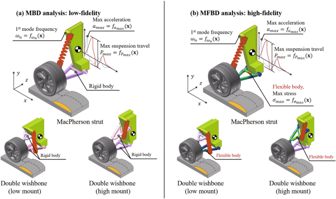
MBD and MFBD analysis configuration
3.3.4 Finite element model and mesh convergence analysis
As shown in Fig. 8, we conducted a mesh convergence analysis on selected cases to ensure that the finite element model provides accurate stress predictions without unnecessary computational expense. The convergence study assesses how the results stabilize as the mesh density increases, allowing us to select an optimal mesh size that balances accuracy with computational efficiency.
Finite Element Model Details: The material properties used in the finite element model are based on SAE 9255 steel, a common material in automotive suspension systems. Young’s modulus (E) is set to 210 GPa, and Poisson’s ratio () is set to 0.3. The finite element model explicitly targets the suspension components most likely to experience high stress. The stress component used for evaluation in this study is the von Mises stress, which provides a scalar value suitable for assessing yield failure in ductile materials.
Mesh Convergence Study: For the mesh convergence study, we selected several representative cases and varied the mesh size across a range from coarse to fine (as shown in Fig. 8). The convergence was evaluated based on the von Mises stress values in the lower arm of each suspension type. Mesh densities were systematically refined, and the corresponding degrees of freedom (DOF) were plotted on a logarithmic scale to observe the stabilization of stress values.
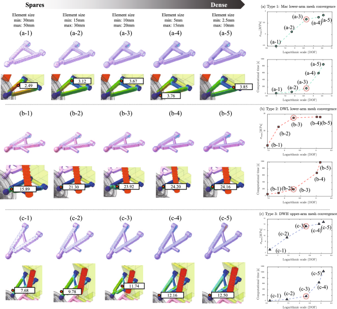
Mesh convergence study for suspension models: Mac (a), DWL (b), and DWH (c). Each model is analyzed with varying mesh densities from sparse to dense. Convergence plots on the right show the relationship between mesh refinement (DOF, logarithmic scale) and key metrics: and computational time
As shown in Fig. 8, this study illustrates the convergence of von Mises stress for each mesh size, highlighting the trade-off between stress and the computational cost. Cases (a), (b), and (c) correspond to the lower arm of the MacPherson strut, double wishbone low mount, and double wishbone high mount types, respectively. By performing MFBD on several design samples with varying mesh sizes, we observed that the von Mises stress began converging from the third mesh condition. However, we also noted that the computational cost increased exponentially with finer meshes. Therefore, in this study, we selected the mesh conditions shown in Fig. 8 (a-3), (b-3), and (c-3) for each suspension type, as these provided a balance between computational efficiency and accuracy in capturing stress behavior.
3.4 Stage 4: Multi-fidelity surrogate model
Stage 4 focuses on training a multi-fidelity surrogate model to efficiently predict the dynamic performance metrics(, , ) of each type of suspension mechanism and the maximum stress() of flexible bodies(in Fig. 9). However, since the defined four performances exhibit non-linearity due to the geometric complexity of each suspension type, we opt for the multi-layer perceptron (MLP) approach. The ability of MLP to capture the nonlinear relationships between design variables and performance metrics provides significant advantages in the engineering domain.
MF model diagram
3.4.1 Low-fidelity model
The low-fidelity model focuses on predicting three performance metrics using the independent design variables () and MCK parameters as inputs(in Fig. 9 (a)). These metrics include , , and . Utilizing the low-fidelity analysis results obtained in Stage 3, the low-fidelity model provides a first approximation of the suspension performance metrics.
The low-fidelity model is implemented as a multi-layer perceptron (MLP) with an input layer, four hidden layers, and an output layer. The input consists of independent design variables (Table 1) and three MCK parameters (Table 2). The architecture of the MLP model is as follows:
where is the total number of hidden layers determined through the AutoML process, and and represent the weights and biases of each layer, respectively.
The loss function for training is the mean squared error (MSE) between the predicted and true performance metrics:
An Adam optimizer is used to update the weights and biases of the model to minimize the loss function. The training process adapts dynamically to the framework requirements, and the optimized model is saved for subsequent analysis. The hyperparameters for the low-fidelity model, including the number of hidden layers and nodes, are determined later through an AutoML process involving multiple iterations (He et al. 2021). This approach focuses on establishing a generalizable design methodology rather than achieving complete optimization of each hyperparameter. While the selected hyperparameters ensure effective performance, absolute optimization is not guaranteed, as the primary aim is to maintain the frameworks flexibility and practical applicability within the design context.
3.4.2 Multi-fidelity model
To effectively integrate the low-fidelity analysis (MBD) with the high-fidelity analysis (MFBD), the density-based spatial clustering of applications with noise (DBSCAN) algorithm was utilized (Yi et al. 2020). This approach enabled the extraction of a representative subset of samples from the MBD results. Specifically, a total of 5 of the samples from the set , which was utilized in the low-fidelity analysis, were selected for the MFBD. The representative samples, , was then utilized for the MFBD, ensuring that the most informative and diverse samples were sampled while ensuring computational costs remained within an acceptable range.
The multi-fidelity model enhances the predictive capability by utilizing the outputs of the low-fidelity model as supplementary inputs. In particular, the multi-fidelity model employs the independent design variables (), MCK parameters, and the three performance metrics predicted by the low-fidelity model to not only anticipate the aforementioned performance metrics (, , and ) but also to project the maximum stress value () in the flexible body (in Fig. 9 (b)). This approach addresses the limitations of the low-fidelity model by refining the predictions of performance metrics that exhibit discrepancies between low-fidelity and high-fidelity analyses and by providing predictions for performance metrics that cannot be obtained from low-fidelity analysis alone.
The multi-fidelity model is structured as a combined neural network, where the output from the low-fidelity model, represented as , is concatenated with high-fidelity inputs, , to form the complete input for the high-fidelity model. Thus, the combined input for the high-fidelity model is:
The high-fidelity model itself consists of several fully connected layers with ReLU activation functions. The hidden layers have 64, 128, 64, and 32 nodes, respectively, with computations defined as:
where represents the total number of hidden layers, dynamically determined using the AutoML process. Here, and are the weights and biases of each layer, respectively. The final output layer predicts high-fidelity performance metrics, including and , based on the transformed inputs. The loss function for training the multi-fidelity model is formulated as the mean squared error (MSE) between the predicted and true high-fidelity performance metrics:
where denotes the number of training samples used in the multi-fidelity analysis, represents the true high-fidelity performance metric, and is the predicted output of the multi-fidelity model. The Adam optimizer is employed to train the model, enabling efficient and adaptive parameter updates across the combined network, thus balancing computational efficiency with predictive accuracy in this complex design framework.
3.5 Stage 5: Design optimization
The aim of Stage 5 is to optimize the performance metrics of each suspension type. Due to the need for multiple evaluations during the optimization process, we utilize the multi-fidelity model trained in Stage 4 to predict performance values for these evaluations. The proposed application focuses on four performance metrics: , , , and . However, for vehicle suspension systems, the first natural frequency mode () is used as a reference performance metric rather than an objective function. This is because the natural frequency is crucial for understanding the dynamic behavior and potential resonance issues of the suspension system. A suspension system with a natural frequency that matches the frequency of road irregularities can lead to resonance, causing excessive vibrations and reduced ride comfort. Therefore, while is not directly optimized, it is monitored to ensure it falls within an acceptable range that avoids resonance with common driving conditions. This approach helps in designing a suspension system that balances ride comfort, stability, and structural integrity without explicitly optimizing the natural frequency as a performance metric. Thus, the optimization problem is formulated as a multi-objective optimization (MOO) problem with three performance metrics (, , and ) as objective functions.
To solve this optimization problem, we use the well-known non-dominated sorting genetic algorithm (NSGA-II) algorithm as the optimizer, using the Python package pymoo (Blank and Deb 2020). The objectives, constraints, and settings for NSGA-II are as follows:
3.5.1 Design variables
The independent design variables for each type of suspension mechanism, as defined in Stages 1 and 2 (in Fig. 2 and Table 1), are as follows: , , and . Additionally, the MCK parameters (in Table 2) are considered in the optimization process. The design variables for each type are defined as combinations of mechanism design variables and MCK parameters: , , and for the respective suspension types. These combined design variables allow for the simultaneous optimization of both each type of suspension and the shock absorber’s mechanical properties. In some cases, specific values could be fixed or design ranges provided to perform optimal design tailored to different performance requirements.
3.5.2 Objective functions and constraints
In the optimization process, the objective functions are defined based on the predicted performance metrics , , and . represents the predicted maximum suspension travel. This value is a crucial indicator of the suspension’s ability to absorb shocks and maintain stability. A lower value of suggests better performance in limiting excessive suspension movement, contributing to vehicle stability and passenger comfort. denotes the predicted maximum acceleration experienced by the suspension mount. This metric is essential for evaluating ride comfort and the structural impact on the vehicle. Minimizing is desirable as it indicates smoother ride quality and reduced peak forces transmitted to the vehicle’s structure. is the predicted maximum stress within the flexible body components of the suspension. This performance metric is critical for ensuring the durability and reliability of the suspension system. Lower values of indicate that the suspension components can withstand operating loads without experiencing high stress, thereby enhancing longevity and safety. Thus, , , and are defined as objective functions to minimize.
The number of constraints for optimizing each type of suspension using the multi-fidelity surrogate model is as follows: , , and . Although the design parameters for each suspension type are not shared, the performance metrics obtained from MBD and MFBD analysis are the same. Therefore, the boundary conditions for the objective function of each optimization are outlined in Eq.(17),(18), and (19). To ensure that the optimization does not escape the design variable range used in training the surrogate model, the design variables for optimization are proposed within the range utilized in the LHS. of the designs are filtered out as outliers to bypass the singularity of the . We used a z-value of 1.95, assuming a normal distribution. Finally, to recommend the optimized design variables for each type based on the input sprung mass (), a boundary condition is applied to restrict the range of the within the MCK conditions. Therefore, each type of suspension optimization problem can be formulated as follows:
The optimization formulation for the Mac type is expressed as:
where is a threshold value used to create a boundary condition by adding to or subtracting from . In the optimization problem handled in this framework, the range of the sprung mass is set narrowly to focus on exploring the optimal solutions for other design variables.
The optimization formulation for the DWL type is expressed as:
Finally, The optimization formulation for the DWH type is expressed as:
Each design variable is constrained within the ranges defined by the LHS boundary provided in Table 1 and Table 2. This ensures that all optimization variables respect the specified design bounds.
The formulation ensures that the optimization process respects each suspension type’s mechanical constraints and objective functions.
4 Results and discussion
4.1 Dynamic analysis (MBD, MFBD) results
In Stages 1 and 2, a total of 35,450 low-fidelity analyses (MBD) were conducted using 300 (Mac), 209 (DWL), and 200 (DWH) samples for each suspension type, respectively, across 50 MCK conditions. The automated dynamic simulation process is summarized as follows: 1) The 3D CAD models generated in Stage 2 are imported, 2) The imported components are automatically assembled according to the joints calculated in Stage 1, and 3) MCK conditions and speed bump road references are assigned to the assembled models, followed by the MBD analysis.
Since constructing the multi-fidelity surrogate model requires high-fidelity (MFBD) samples, and given the computational expense, using all MBD samples for MFBD analysis is impractical. Typically, only to of high-fidelity analyses are performed, depending on the application. Therefore, selecting a representative subset from the MBD results is critical for building a robust multi-fidelity model that balances computational cost and model accuracy. The design variables for the MBD analysis were sampled using LHS, as shown in Tables 1 and 2. However, because the performance metrics obtained from MBD are not evenly distributed across the performance space, using LHS directly would not ensure representative sampling for MFBD analysis. Instead, we analyzed the distribution of the MBD results to identify high-density and low-density regions in the performance space via DBSCAN (in Fig. 10).
To capture both the diversity and representativeness of the samples in this non-uniform distribution, we employed the Density-Based Spatial Clustering of Applications with Noise (DBSCAN) algorithm. Unlike clustering methods like k-means, which require specifying the number of clusters in advance, DBSCAN is advantageous because it identifies clusters based on density rather than pre-defined cluster numbers. By setting a minimum sample size and a radius parameter, DBSCAN detects dense clusters in the performance space, allowing us to select samples from each region systematically. This approach ensures that high-density areas are not overrepresented while ensuring adequate representation in low-density areas. As shown in Fig. 10, DBSCAN selected of the MBD samples, yielding a set of MFBD samples more evenly distributed across the normalized performance metrics (Ester et al. 1996). This sampling process enables the construction of a multi-fidelity model that effectively captures the variations in both high- and low-density regions of the performance space, providing a balanced dataset for training.
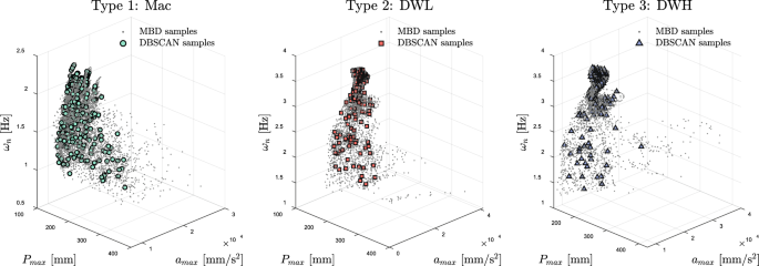
MBD samples and DBSCAN samples configuration
The MFBD analysis of the samples selected via DBSCAN obtained four performance metrics (, , , ). Before constructing the multi-fidelity surrogate model, a comparison of three performance metrics (, , ) between MBD and MFBD analyses is shown in Fig. 11. The x-axis represents values from the MBD analysis, and the y-axis represents values from the MFBD analysis. The closer the scatter plot is to the line, the smaller the difference between MBD and MFBD analyses. To quantitatively compare the three performance metrics for each type, we calculated the Mean Absolute Percentage Error (MAPE) using Eq.(20). MAPE effectively expresses the ratio of multiple data values to errors, making it useful for analyzing trends across various samples, as shown in Fig. 11. The MAPE results for the MBD and MFBD analyses are presented in Table 3.
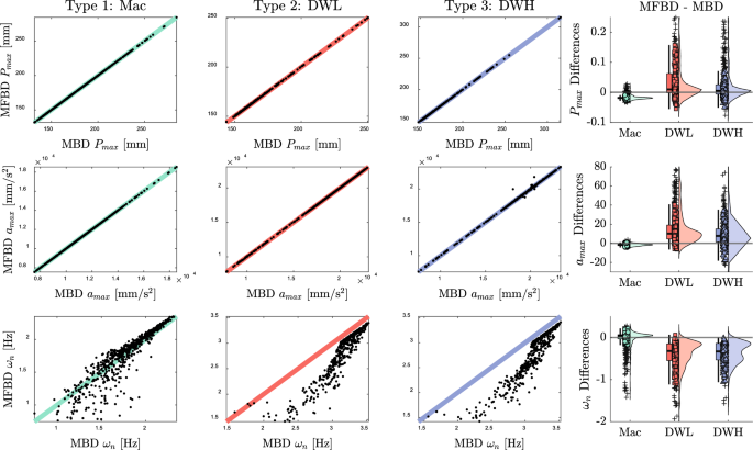
MBD vs MFBD results comparison
The metrics for and are nearly indistinguishable between the MBD and MFBD analyses, indicating that the results are so closely aligned that additional high-fidelity analyses may be unnecessary for these specific metrics. However, while showing a similar overall trend, the metric exhibits significant differences in certain cases. This discrepancy is consistent with the finding that the natural frequency of mechanisms assumed to be rigid can be significantly affected when specific parts are modeled as flexible bodies using finite element analysis (Kim et al. 2019).
Given these observations, the low-fidelity analysis (MBD) and the representative samples from DBSCAN were used to confirm the similarities in and values across different fidelity types. Consequently, for constructing the multi-fidelity model predicting all four performance metrics, and are derived directly from the low-fidelity model, while and are predicted using the high-fidelity analysis.
The multi-fidelity model is designed to predict four performance metrics by combining the outputs from both the low-fidelity and high-fidelity models. The low-fidelity model initially predicts three performance metrics, , , and :
where represents the low-fidelity predictive model, with as its input design variables and MCK parameters.
Out of these low-fidelity predictions, and are used as supplementary inputs in the high-fidelity model. These two outputs, denoted
are concatenated with high-fidelity inputs, , to form the input for the high-fidelity model. The high-fidelity model then predicts and , which require higher accuracy:
where represents the high-fidelity predictive model, leveraging the concatenated inputs to improve prediction accuracy.
The final combined output of the multi-fidelity model, denoted as , incorporates all four performance metrics:
This combined approach enables the multi-fidelity model to deliver a comprehensive performance prediction, utilizing the low-fidelity model’s efficiency for certain metrics and the high-fidelity model’s precision for metrics that demand detailed analysis.
4.2 Multi-fidelity model prediction results
To construct the multi-fidelity (MF) model, it is essential to first train the low-fidelity (LF) model (in Fig. 9). To avoid overfitting during the training of the LF model for each suspension type, an AutoML approach was employed to iterative optimize the hyperparameters. Once the LF model was successfully trained, it served as the foundation for developing the MF model. The MF model was trained using of the samples selected through DBSCAN and the pre-trained LF model.
As indicated in Fig. 11 and Table 3, and show almost identical results between MBD and MFBD analyses; therefore, these metrics were not separately predicted in the MF model. However, exhibited significant differences between MBD and MFBD analyses, making it necessary to predict this metric within the MF model to capture the dynamic behavior accurately. Additionally, is a metric that cannot be obtained through MBD analysis alone, as it requires the flexible body dynamics offered by MFBD. Consequently, is also predicted within the MF model to provide a comprehensive assessment of the suspension’s structural performance. In Fig. 12 and 13, the x-axes represent the ground truth values: for Fig. 12, the low-fidelity (MBD) data, and for Fig. 13, the high-fidelity (MFBD) data. This distinction clarifies the comparison between the predicted and actual values within each fidelity level and supports the validation of the MF model’s performance across different metrics.
The computational environment, hyperparameters used for training the LF and MF models, and the accuracy of the predictions, including the performance of the MF models trained using the samples selected via DBSCAN, are summarized in Table 4, and Fig. 12, 13. The accuracy of the predictions was evaluated using R-squared (), Mean Squared Error (MSE), and Root Mean Squared Error (RMSE), providing an objective comparison between the models. Given that most of the trained MLP predictions are similar to the corresponding ground truth values, the MLP model has been trained successfully.