Article Content
Abstract
The increasing population and future drought scenarios caused by climate change require research into new integrations between technologies, such as remote sensing and water productivity models, to optimize the use of water resources in agriculture and strengthen food security. Peru, the world’s leading quinoa producer, considers this crop of great interest due to its nutritional value, adaptability, and resistance to water stress. This study is proposed to establish irrigation thresholds based on the crop water stress index (CWSI) and the AquaCrop model, previously calibrated with the volumetric soil moisture (θ) and canopy cover (CC) of the Amarilla Marangani mutant line quinoa variety during the cold season in which quinoa is most cultivated in Peru. Canopy temperature was monitored with an IR thermal camera, CC with a digital camera, and θ with a TDR-300 sensor. The crop underwent stepwise irrigation reductions (50, 75, and 100% ETc) under a drip irrigation system and a control treatment (full ETc). A significant linear relationship (p < 0.05) was found between CWSI and θ, which allowed us to estimate the water status of the crop accurately. In addition, the AquaCrop model showed a “very good” to “good” performance in the simulation of CC, θ, biomass, and yield development. Activating irrigation at a CWSI of 0.44 is recommended, equivalent to the water consumption of 2770 m3 ha−1, achieving a 29% water saving and a yield of 2.5 t ha−1. These results highlight the potential of combining technologies to improve irrigation efficiency in arid areas and have agricultural sustainability options in the face of climate change.
Explore related subjects
Discover the latest articles and news from researchers in related subjects, suggested using machine learning.
- Agricultural Geography
- Agriculture
- Agronomy
- Crop waste
- Drought
- Subsistence Agriculture
Introduction
Climate change and population growth put additional pressure on resources vital for agricultural production, such as water availability [28]. Therefore, efficiently managing drought-tolerant crops such as quinoa is essential for sustainable agricultural production in regions with water scarcity [4].
This research was carried out in the district of La Molina in Peru, characterized by a temperate climate, with intense sun between January and March and scarce drizzle the rest of the year. Therefore, efficient water use in drought-tolerant crops is necessary to achieve irrigated agriculture. In this sense, recognizing water stress thresholds and irrigation management via infrared thermography and the AquaCrop water productivity model is an alternative to optimize irrigation programming and achieve more significant water savings and increased yields [21].
Quinoa (Chenopodium quinoa Willd.) is a crop with high nutritional value and protein quality that provides essential amino acids [14, 20]. In addition, it has a high tolerance to water stress, a vital rotation alternative in arid and FAO semi-arid zones [13]. The FAO also recognized it in 2013 as the grain that will combat hunger and malnutrition and safeguard food security [1]. The average world production of quinoa from 2015 to 2022 was 164,055 t, with Peru being the leader, with a production of 58.7%, followed by Bolivia (38.9%) and Ecuador (2.4%) [7].
According to [13], Peru has 3000 quinoa accessions, with 20 varieties being the most cultivated, in the departments of Puno, Ayacucho, and Apurímac, their growth being possible due to the different agroecological levels. The largest area is located above 3000 m above sea level, especially in the fields of small-scale farmers, ensuring high-quality production in rainfed conditions, periods of drought, low temperatures (falls below zero, going down to − 30 °C), rainfall from 0 to 1000 mm, also, in soils with low fertility, pH (4–9), and salinity problems [13].
Improving crop productivity requires understanding the biophysical variables influencing crop yield [23]. With respect, the FAO AquaCrop model makes it possible to predict crop yield through a water productivity model that simulates biomass production based on the amount of water transpired from the plant cover, allowing optimization of crop yield, even in limiting conditions of water and temperature, key in production [23]. In consistency, the CWSI is a function of the difference between the canopy temperature and the air temperature (Tc–Ta) and the vapor pressure deficit (VPD), being a good indicator of the water status of the plant since the leaf temperature is representative of the stomatal conductance [22]. Hence, applications such as the AquaCrop model and the CWSI would improve the planning and monitoring of water management in situations of water stress linked to production. This study aims to propose thresholds for the time of irrigation based on information from remote sensing and the AquaCrop model, previously calibrated, to present new irrigation programs that allow water savings using the mutant line of quinoa derived from Amarilla Marangani variety in irrigation systems on the central coast.
Materials and Methods
Place and Design of the Experiment
The experiment was developed in the Cereals and Native Grains Program of the La Molina National Agrarian University (12° 04′ 42″ S and 76° 56′ 37″ W, altitude 251 AMSL) located in the district of La Molina, the province from Lima, on the central coast of Peru, which is located in the ecological formation «subtropical desiccated desert» (dd-S) according to Holdridge’s classification of life zones. Average annual temperature, relative humidity (RH), and precipitation were 19.9 °C, 75.8%, and 28.1 mm, respectively.
The treatments consisted of irrigation equal to the ETc (control, T0) and irrigation with a staggered reduction of 50%, 75%, and 100% of the ETc (T1). Eight experimental units of 1.2 m × 7 m correspond to these two treatments, distributed in 4 repetitions per treatment. The water was supplied under drip irrigation through polyethylene laterals of 16 mm in diameter, with an average discharge of emitters of 1.4 L h−1 and distance between drippers and lines of 0.30 m and 0.60 m, respectively (Fig. S1).
Crop Management and Phenology
The quinoa variety was the “mutant line of Amarilla Marangani variety” (MQ-AM 250-283), with manual sowing in winter, a continuous stream, and two rows separating 0.6 m, with a sowing density of 18 g of seed per row. A fertilization dose of NPK of 40-60-0 was applied during sowing, and another dose of 40-0-0 was applied 54 days after sowing (DAS) at the beginning of flowering. These are within the agronomic recommendations of fertilization and planting density according to the FAO manual “Quinoa Cultivation Guide” [12]. Likewise, [13] mentions that crops with the highest yield have a plant population evenly distributed throughout the field, with approximately 400,000–500,000 plants/ha, so we adjusted to a density of 452,500 plants/ha.
Figure 1 presents the characterization of the phenology according to the classification criteria of [26] and from the FAO in DAS and growing degree days (GDD). The most significant growth phase occurred in the anthesis with an average height of 153 cm at 86 DAS. The aqueous grain phase occurred at 86 DAS, a phase-sensitive to drought, achieving physiological maturity at 128 DAS, and then proceeding to harvest, obtaining the yield and biomass according to the procedure described by [13].
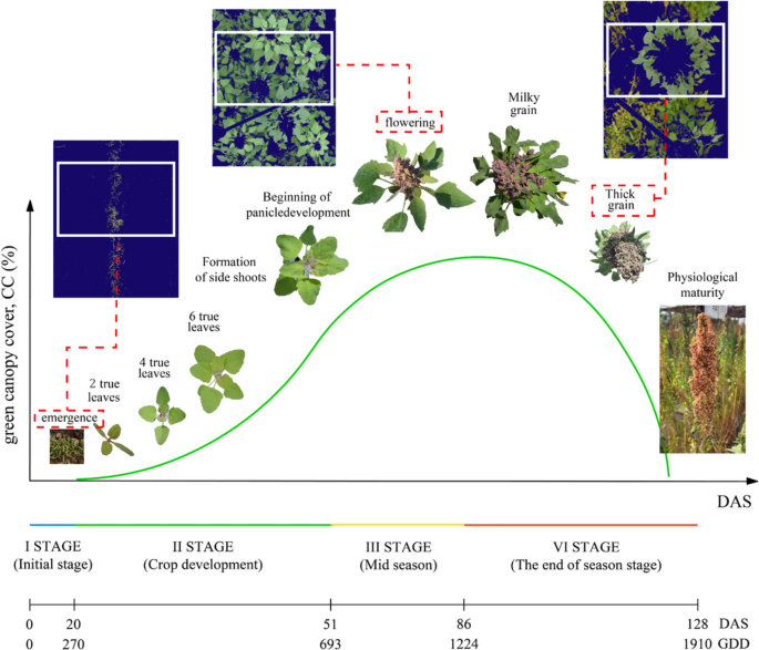
Representation of canopy cover growth
Characterization of Irrigation Water and Soil
The irrigation water had a pH of 8.16, an electrical conductivity of 0.62 dS m−1, Ca++ of 4.53 meq L−1, Na+ of 0.83 meq L−1, Mg++ of 0.66 meq L−1, resulting in a RAS of 0.52 and classification C2- S1 according to Richard’s diagram. The soil texture was sandy clay loam (51% sand, 26% silt, 23% clay); θ at field capacity and wilting point was 25.4 and 14.0%, respectively, bulk density of 1.25 g cm−3, with a low percentage of organic matter, low cation exchange capacity (CEC), medium content of phosphorus and potassium, being, in general, a soil of low natural fertility.
Evaluations
Canopy temperature
For the study, a thermographic camera, model E60, manufactured by FLIR Systems (Wilsonville, USA), was used to obtain thermal and optical images with dimensions of 320 × 240 and 2048 × 1536 pixels, respectively. The images record temperature measurements in the range of 7.5–13 µm, with a frame rate of 60 Hz, and have an accuracy of ± 2 °C and a thermal sensitivity of 0.05 °C. In addition, 6 “T”-type thermocouple (TTS) thermal sensors (positive copper cable and negative constantan cable, copper and nickel alloy, joined by tin welding) of the OMEGA brand, model TT-T-36- were used. SLE-500 is installed in the crop canopy with data storage through the PC200W collector, Campbell Scientific brand.
The canopy temperature (Tc) was measured between 13 and 14 h of the day, in the open air, in a west–east direction, at a distance of 1 m above the crop canopy, with an angle of 90° and adjusted to an emissivity of 0.96. The canopy cover was identified with the true-color optical image, and the Tc was obtained with the thermal image (Fig. 2).
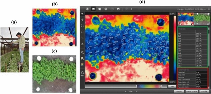
a Image capture at 1 m above the crop canopy, b thermal infrared image, c actual color image, d FLIR Tools program panel with parameters
Humidity of Soil
Immediately after collecting the images, soil moisture measurements were taken at a depth of 0.20 m using a TDR-300 (Field Scout) portable moisture sensor, with readings before and after irrigation, previously adjusted with gravimetric samples and bulk density to obtain θ and estimate the water depth in the soil (Wr).
Canopy Cover
The CC was evaluated weekly with six monitoring repetitions (Fig. S2) via aerial photographs captured from the top (Fig. 1p). These images were processed with the Easy Leaf Area software [5]; then, the green cover of the canopy was divided concerning the reference area of 1800 cm2, obtaining the CC percentage.
Crop Water Stress Index (CWSI)
The VPD was obtained from the temperature and RH of the air available at the Alexander Von Humboldt weather station. By plotting (Tc–Ta) versus VPD, the lower limit (LL) was obtained, which represents a state of transpiration without water stress. The upper limit (UL) is an independent horizontal line of the VPD that describes the situation of maximum water stress (absence of transpiration). The temperature difference (Tc–Ta) relationship versus the VPD for the LL was determined with the information collected at T0. For the UL, the information obtained from T1 was used. The CWSI is defined under the following equation [4] (Eq. 1):
where canopy and air temperatures are Tc and Ta (°C).
Calibration of AquaCrop Model
Sensitive model parameters such as normalized water productivity (WP*), CC max, canopy decline coefficient (CDC), and canopy growth coefficient (CGC) were calibrated. They have compared the variables CC and Wr observed and simulated, relating them linearly to evaluate the performance of the model through different statistical indicators such as the Nash–Sutcliffe efficiency (NSE), normalized mean square error (NRMSE), the ratio of standard deviation (RSR), and Wimbolt’s index (d). With these indicators, the model’s efficiency was identified according to the rating scale proposed by [19]. Pearson’s correlation (r) was also obtained with the Student’s t statistic test for an alpha significance level of 5%.
Furthermore, [2] and [9] mention that hot or high-temperature seasons in desert areas can negatively influence yield during the development or flowering period in quinoa crops. Therefore, the calibration of the AquaCrop model was carried out only in the cold season, when quinoa is most cultivated in Peru. This allows parameters to be adjusted to the most representative season of the region, providing a solid basis for simulations in similar scenarios. Still, it is essential, according to [15], to validate in multiple seasons to capture interannual variability and improve the robustness of the model.
Results and Discussion
Irrigation Applications and Treatments
Figure 3a shows the irrigation film (IF) applied during crop development. To T1, a reduction in irrigation was used in a staggered manner (50%, 75%, and 100% of the ETc) at 93, 100, and 109 DAS, and the final volumes of applied water of 2770 m3 ha−1 and 2090 m3 ha−1 for T0 and T1, respectively, representing a 25% reduction of T1 compared to T0, because the milky grain phase is the most sensitive in quinoa [10]. The IF reduction treatments were carried out at the beginning of this phase (93 DAS), with staggered irrigation reductions, intending to cause water stress in the crop.
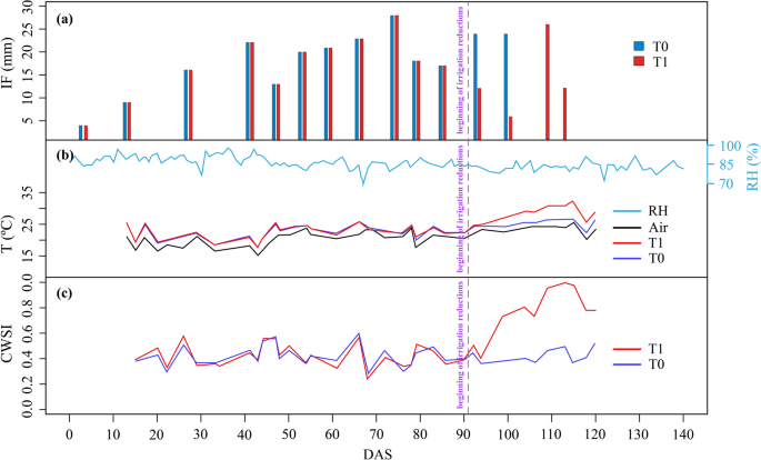
Temporal variation of a irrigation film; b leaf temperature, air temperature, and relative humidity; c CWSI
Furthermore, through the analysis of variance (ANOVA), the averages of biomass and yield between treatments T0 and T1 were compared. There were no significant differences since their p-values were higher than the significance level (α = 0.05).
Accordingly, the reduction of irrigation in the initial phase of milky grain (93 DAS) until harvest turned out to be less severe than to reduce crop yields significantly, possibly because the irrigation reduction was staggered, giving the crop time to adapt. In addition, it has been reported that high RH favors the calcium oxalate present in quinoa leaves, being able to absorb water from the environment, keeping the leaf turgid and the photosynthetic rate high (high stomatal conductance) in drought conditions. In addition, transpiration losses are kept at low levels, thus improving their tolerance to water stress [10, 15].
Canopy Cover and Soil Moisture Content
Figures 4 and 5 show the fit between observed and simulated data regarding CC and Wr, which obtained a strong correlation of 0.96 and 0.86 on average, respectively, with the Student’s t test for a 5% alpha level. The model represented the CC well from the phenological period from sowing to the milky grain (93 DAS). From this phase, Fig. 4b shows the decrease in Wr due to the irrigation cut made in T1.
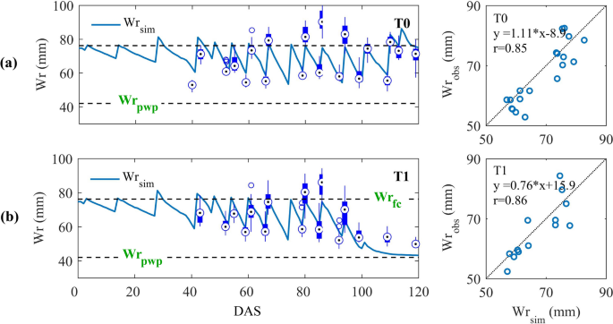
Observed and simulated Wr of the quinoa crop of the MQ-AM variety under treatments a T0 and b T1
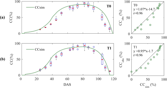
Observed and simulated CC of the quinoa crop of the MQ-AM variety under treatments a T0 and b T1
Furthermore, the model represents the Wr below the observed data as the humidity decreases; even so, in this period, it did not cause a more significant difference or reduction in CC between treatments, as seen in Figs. 5a, b. In general, following the classification according to [19], this model had a “very good” performance for CC and “good” for Wr, by what was obtained by various statistical indicators such as RSR, NRMSE, NSE, and d.
AquaCrop Calibrated Parameters
Table 1 shows the values of the calibrated parameters of the MQ-AM variety. The values for the upper temperature (Ts) of 30 °C were conservative parameters according to [14] and the base temperature (Tb) of 3.3 °C according to that obtained by [3] and with which the Tb of Amarilla Marangani variety was determined in the most critical stage (flowering). The plant density was 452,500 plants/ha, within the range recommended by [13] of 400,000–500,000 plants/ha to obtain higher yields. The CGC calibrated in T0 and T1 was 8.5 and 9.2% d−1, respectively; thus, the T1 presenting higher CGC had slightly more ability to expand its canopy up to 9.2% per day. The CCx was 93 and 90% for T0 and T1, respectively, while [9] and [6], due to having a lower planting density and more space between crops, calibrated their models with 70 and 75%, respectively. The CDC was calibrated at 8.9 and 9.1% d−1 (0.557 and 0.573% GDD−1) for T0 and T1, respectively, without showing differences in CDC between the treatments. For this reason, the reduction in irrigation, since it was not so severe, did not allow us to offer a marked decrease in canopy cover, which, in the end, is the normal physiological response of the crop to water deficit [13].
The WP* was set at 13 g m−2 for the T0 and T1 treatments, respectively, being higher than the one calibrated by [9] between 9.3 and 10.4 g m−2, which better explains its efficient use of water as it is the MQ-AM variety, an improved line in the face of drought; also [24] obtained very similar water productivity values between 11.8 and 13.4 g m−2. The water stress parameters were maintained with the values proposed by [9]. In addition, the shape factor (fs) is 4, indicating that crop development is only affected when water stress becomes severe.
It is essential to highlight that to generalize the use of these calibrated parameters in other varieties of quinoa, geographic locations, seasons, irrigation treatments, or agronomic factors, according to [9] and [15], they highlight the importance of validating the models in multiple scenarios to capture the interannual and environmental variability, because in their research they have shown that climatic conditions and irrigation management can significantly affect agricultural yields.
CWSI Stressed and Non-stressed Baseline
Figure 6 shows the hourly variation of Ta and Tc, measured with TTS at 109, 113, and 115 DAS between 9 and 17 h. It is observed that the Tc follows a bell curve trend, reaching maximum values between approximately 13 and 14 h. [4] An optimal time to evaluate the CWSI is clear skies and sunshine. For this reason, all the CWSI evaluations were carried out between 1:00 and 2:00 p.m.
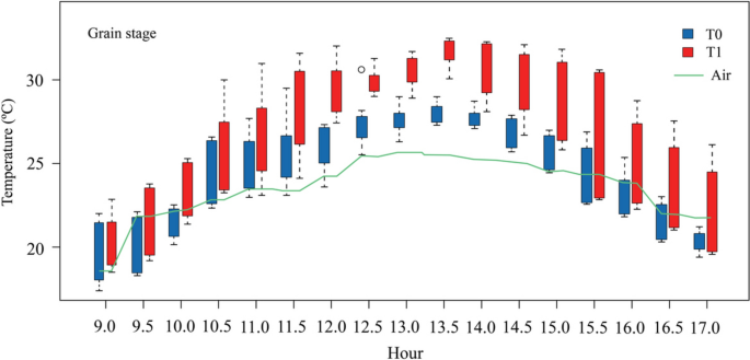
Hourly Tc and Ta variation measured with TTS at 109, 113, and 115 DAS
Figure 7 shows the equations of the UL and LL for the situations of maximum and minimum stress, respectively, developed for the calculation of the CWSI according to the empirical approach recommended by [4]. A UL = 7.1 was obtained, representing the difference between Tc and Ta when there is no crop transpiration (maximum stress). This line is a constant function that does not depend on the VPD. In this regard, in a similar investigation in Turkey by [4] in the quinoa crop, cv, Titicaca obtained an upper limit of 4.75 °C. The LL was developed for three representative stages of growth.
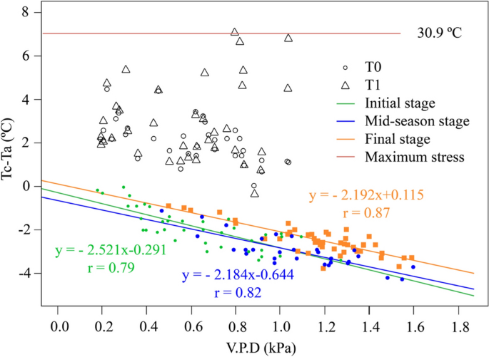
Baselines of maximum and minimum stress, according to the relationship between the temperature difference (Tc–Ta) and VPD during the growth stages of the crop
It was obtained LL = − 2.521VPD − 0.291 for the initial stage (vegetative phase, flower bud, and inflorescence), LL = −2.184VPD-0.644 for the mid-season stage (flowering phase and anthesis), and LL = − 2.192VPD + 0.115 for the final stage (watery, milky, and pasty grain phase), obtaining Pearson’s correlation coefficient (r) of 0.79, 0.81, and 0.87, respectively, and with a p-value < 0.05 for each case, thus showing a high and significant correlation. These LL equations show slight changes in the slope and intercept of the line, which can be summarized in the following equation: LL = (−2.521–2.184) VPD + (−0.644 + 0.114). Bozkurt et al. [4] reported a similar equation for all the phenological phases of the quinoa crop (LL = −1.4952 VPD + 1.351).
The baseline without water stress varies according to the crop, phenology, and climatic conditions [25]. The VPD throughout the evaluation period remained in a low range (0.18 to 1.60 kPa), which indicates that the air can retain large amounts of water vapor in the environment, thus generating an average RH of the air elevated in the environment, as can be seen in Fig. 3b, where the RH varied from 69 to 98%.
Figure 3b shows the variation in time (11 to 120 DAS) of Tc, Ta, and RH. Once the water cut started at 93 DAS, an increase in the Tc of the T1 treatment is observed in comparison with the Ta, reaching a maximum gain of 28.5%, registered 25 days after the water cut (113 DAS, when the water content was reduced to 100%). A maximum Tc was recorded for the quinoa crop (32.2 °C) higher than Ta at 7.1 °C (maximum difference between Tc and Ta). In a similar investigation [4] in the quinoa crop, cv.Titicaca obtained a maximum difference of 4.75 °C, possibly due to the differences in the crop variety, the climatic conditions, and the soil in which the experiment was conducted. With the maximum difference found (7.1 °C), the UL was developed, similar to the procedure recommended by other authors [17]. The difference between the current Tc and Ta is located within the LL and UL, thus obtaining the necessary information for calculating the CWSI.
CWSI and Soil Moisture
Figure 3c shows the variation of the CWSI concerning the DAS for the two treatments (T0 and T1). Before 93 DAS (beginning of the irrigation cut, milky grain phase), both treatments follow a similar CWSI trend; after 93 DAS, an increase in the CWSI is observed in T1, given the staggered reductions in irrigation of 50%, 75%, and 100% of the ETc, and performed at 93, 100, and 109 DAS, respectively. T1 reached a CWSI of 1 (maximum stress) 22 days after the start of the water cut, while the CWSI of T0 was 0.495.
Figure 8 shows the relationship between CWSI and θ%. It is observed that values of CWSI < 0.61 correspond to values of θ % > 17.29%, with the relationship θ % = 39.312 − 36.104CWSI (r2 = 0.832, r = −0.912 with p-value < 0.05 in the F test—Fisher), while for CWSI values > 0.61, they correspond to θ% values < 17.29%, with the relationship θ % = 19.716 − 4.2258CWSI (r2 = 0.503, r = −0.709, with p-value < 0.05 in the F—Fisher test), demonstrating in both cases an inverse and significant correlation.
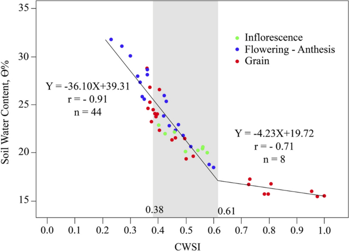
Relationship between CWSI and θ
The relationship between the CWSI and θ demonstrates the validity of using non-contact thermal detection to measure soil moisture (θ) indirectly; therefore, using irrigation scheduling techniques based on the CWSI is recommended. According to the results obtained, the suggested CWSI value for optimal irrigation of the MQ-AM variety of quinoa is in the range of 0.38 to 0.61, related to a θ range of 25.6% (field capacity) to 17.2%, a value that corresponds to a critical CWSI, from which a 3% decrease in θ generates a 39% increase in CWSI, which demonstrates the sensitivity of the crop from a CWSI of 0.61.
The study applies to the irrigation programming method where the soil water content is known since a significant relationship was obtained between soil moisture and CWSI. With this relationship, a CWSI value is obtained for each soil moisture value, which is why monitoring soil moisture from CWSI is possible. Comparisons have not been made with parameters other than soil moisture to apply other irrigation programming methods. However, there are investigations in other crops where significant relationships have been found between CWSI and biological measurements of the plant, such as sap flow or foliar water potential [12], and with crop evapotranspiration (ETc) [16], which has allowed other irrigation programs to be applied.
Applied Water Use Efficiency (Applied WUE)
Fajardo et al. [6] mentions the positive effect of limiting irrigation on quinoa yield; therefore, reducing the IF applied in T1 improved its WUE from 0.63 to 0.74 at kg m−3 (Table 2).
The results of the simulations with the previously calibrated AquaCrop model, the applied WUE, and WUE were obtained for different levels of irrigation depth and its corresponding average WC (Fig. 9). In this regard, for a yield of 2.5 t ha−1, there is a consumption of 3880 m3 ha−1, equivalent to a CWSI of 0.40; however, if water consumption is reduced up to 29%, the yield is maintained. Therefore, activating irrigation at a CWSI of 0.44 is recommended, equivalent to the water consumption of 2770 m3 ha−1. On the other hand, a maximum WUE applied of 1.0 kg m−3 is achieved, with a yield reduction of 22% but a water saving of 50% (CWSI 0.60). At this level of 50% reduction in irrigation, [8] mentions that the physiological traits of the quinoa plant exhibit an interesting tolerance to water stress.
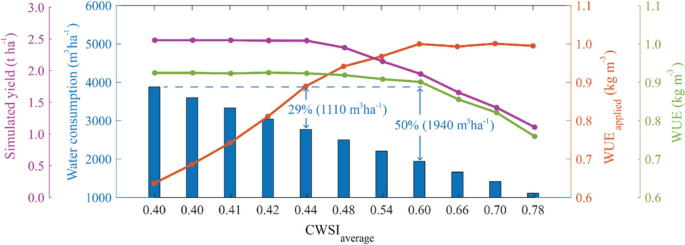
WUE variation, WUE applied, and simulated yield based on average CWSI and water consumption reductions
The CWSI and AquaCrop model results identified irrigation thresholds in the quinoa crop variety (MQ-AM 250-283) developed in an arid area, achieving water savings and improved performance. However, an economic evaluation is necessary to adopt these technologies to achieve a cost-effectiveness ratio.
Conclusions
The CWSI shows that it is a reliable indicator of water deficit in the MQ-AM variety due to its relationship with θ. Obtaining a CWSI < 0.6, the relationship θ = 39.312–36.104 CWSI, with R of 0.912.
The AquaCrop model had a calibration efficiency from “good” to “very good” to simulate canopy cover and soil water content during crop development. The use of the CWSI and the AquaCrop model allows proposing thresholds for the time of irrigation, so it is recommended to activate irrigation at a CWSI in the range of 0.38–0.61, according to soil moisture of 25.6% (θcc) to 17.2%.
For a yield of 2.5 t ha−1, water consumption is 3880 m3 ha−1, corresponding to a CWSI of 0.40. However, this yield is maintained if water consumption is reduced by 29% (CWSI = 0.44).
It is estimated that a maximum WUE applied of 1.0 kg m−3 can be achieved with a water saving of 50% (CWSI 0.60), which could increase agricultural areas in arid zones and mitigate the effect of future drought scenarios.
In the future, thermal imaging is expected to be used in automated irrigation, associated with UAVs, radiofrequency satellite sensors, and ground sensors connected with wireless sensor networks [2]. Many researchers predict further advances in temporal and spatial resolution in satellite remote sensing to achieve daily measurements; additionally, seasonal models will be developed for water stress detection to schedule irrigation [27]. Recent advances in cloud computing and wireless technologies could help process remote sensing data quickly after acquisition [18]. Soon, farmers will benefit from accurate irrigation guidance using instant images from UAVs, weather stations, and direct sensors that can be collected and stored in the cloud and combined with post-processing algorithms to decide advanced irrigation applications [11]. Finally, automation and computational resources will be combined to create innovative technologies for artificial intelligence and real-time processing for decision-making tools. Furthermore, technological advances in the coming years are expected to result in smaller and more affordable devices, making thermal sensing a widespread practice in agriculture, irrigation management, and related fields [2].
Availability of data and materials
The datasets used and analyzed during the current study are available from the corresponding author upon reasonable request.
References
-
Angeli V, Miguel-Silva P, Crispim-Massuela D, Khan MW, Hamar A, Khajehei F, Graeff-Hönninger S, Piatti C (2020) Quinoa (Chenopodium quinoa Willd.): An overview of the potentials of the “golden grain” and Socio-economic and environmental aspects of its cultivation and marketization. Foods 9(2):216. https://doi.org/10.3390/foods9020216
-
Awais M, Li W, Cheema MJ, Zaman Q, Shah A, Aslam B, Zhu W, Ajmal M, Faheem M, Hussain S, Nadeem A, Afzal M, Liu C (2022) UAV-based remote sensing in plant stress: imagine using high-resolution thermal sensors for digital agriculture practices: a meta-review. Int J Environ Sci Technol. https://doi.org/10.1007/s13762-021-03801-5
-
Bertero HD, King RW, Hall AJ (1999) Modeling photoperiod and temperature responses of flowering in quinoa (Chenopodium quinoa Willd). Field Crops Res 63(1):19–34. https://doi.org/10.1016/S0378-4290(99)00024-6
-
Bozkurt Y, Yazar A, Alghory A, Tekin S (2021) Evaluation of crop water stress index and leaf water potential for differentially irrigated quinoa with surface and subsurface drip systems. Irrig Sci 39(1):81–100. https://doi.org/10.1007/s00271-020-00681-4
-
Easlon HM, Bloom AJ (2014) Easy leaf area: automated digital image analysis for rapid and accurate measurement of leaf area. Appl Plant Sci 2(7):1400033. https://doi.org/10.3732/apps.1400033
-
Fajardo H, García M, Raes D, Van Gaelen H (2016) Validación del modelo Aquacrop para diferentes niveles de fertilidad en el cultivo de quinua en el altiplano boliviano. Cintex 21(2):31–52
-
FAO (2024) Faostat: FAO Statistical Databases. Rome, Italy: Food & Agriculture Organization of the United Nations (FAO). Available at http://www.fao.org/faostat/en/#data/QCL/visualize. Accessed July 2024
-
Fghire R, Wahbi S, Anaya F, Issa Ali O, Benlhabib O, Ragab R (2015) Response of quinoa to different water management strategies: field experiments and saltmed model application results: saltmed model testing of deficit-irrigated quinoa production. Irrig Drain 64(1):29–40. https://doi.org/10.1002/ird.1895
-
Geerts S, Raes D, Garcia M, Miranda R, Cusicanqui JA, Taboada C, Mendoza J, Huanca R, Mamani A, Condori O, Mamani J, Morales B, Osco V, Steduto P (2009) Simulating yield response of quinoa to water availability with AquaCrop. Agron J 101(3):499–508. https://doi.org/10.2134/agronj2008.0137s
-
Geerts S, Raes D, García M, Vacher J, Mamani R, Mendoza J, Huanca R, Morales B, Miranda R, Cusicanqui J, Taboada C (2008) Introducing deficit irrigation to stabilize yields of quinoa (Chenopodium quinoa Willd.). Eur J Agron 28(3):427–436. https://doi.org/10.1016/j.eja.2007.11.008
-
Goap A et al (2018) An IoT-based smart irrigation management system using machine learning and open source technologies. Comput Electron Agric 155:41–49
-
Gómez Pando L, Aguilar Castellanos E (2016) Guía de cultivo de la quínoa. Organización de las Naciones Unidas para la Alimentación y la Agricultura (FAO), Rome. http://www.fao.org/3/a-i5374s.pdf
-
Gomez-Pando LR, Aguilar -Castellanos E, Ibañez-Tremolada M (2019) Quinoa (Chenopodium quinoa Willd.) Breeding. In: Advances in plant breeding strategies: cereals. Springer, Cham. pp 259–316. https://doi.org/10.1007/978-3-030-23108-8_7
-
Isobe K, Uziie K, Hitomi S, Furuya U, Ishii R (2012) Agronomic studies on quinoa (Chenopodium quinoa Willd.) cultivation in Japan. Jpn J Crop Sci 81(2):167–172. https://doi.org/10.1626/jcs.81.167
-
Jacobsen SE, Mujica A, Jensen CR (2003) The resistance of Quinoa (Chenopodium quinoa Willd.) to adverse abiotic factors. Food Rev Int 19:1–2. https://doi.org/10.1081/FRI-120018872
-
Katimbo A, Rudnick DR, Zhang J, Ge Y, DeJonge KC, Franz TE, Shi Y, Liang W-z, Qiao X, Heeren DM, Kabenge I, Nakabuye HN, Duan J (2023) Evaluation of artificial intelligence algorithms with sensor data assimilation in estimating crop evapotranspiration and crop water stress index for irrigation water management. Smart Agric Technol 4, 100176, ISSN 2772-3755, https://doi.org/10.1016/j.atech.2023.100176
-
Khorsandi A, Hemmat A, Mireei SA, Amirfattahi R, Ehsanzadeh P (2018) Plant temperature-based indices using infrared thermography for detecting water status in sesame under greenhouse conditions. Agric Water Manag 204:222–233. https://doi.org/10.1016/j.agwat.2018.04.012
-
Lakhwani K et al (2019) Development of IoT for smart agriculture a review. Emerging trends in expert applications and security. Springer, Berlin, pp 425–432
-
Moriasi DN, Arnold JG, Van Liew MWV, Bingner RL, Harmel RD, Veith TL (2017) Model evaluation guidelines for systematic quantification of accuracy in watershed simulations. Trans ASABE 50(3):885–900. https://doi.org/10.13031/2013.23153
-
Ng CY, Wang M (2021) The functional ingredients of quinoa (Chenopodium quinoa) and physiological effects of consuming quinoa: a review. Food Front 2:329–356. https://doi.org/10.1002/fft2.109
-
Nurit A, Yuval C, Jaj B, Victor A, Dilia K, Dilia K, Arnon D, Uri Y, Alon B-G (2013) Una visión del comportamiento del índice de estrés hídrico del cultivo de olivo. Gestión del Agua Agrícola 118:79–86. https://doi.org/10.1016/J.AGWAT.2012.12.004
-
Quezada C, Bastias R, Quintana R, Arancibia R, Solís A (2020) Validación del índice del estrés hídrico de cultivo (CWSI) mediante termografía infrarroja y su incidencia en rendimiento y calidad en manzanas “Royal Gala.” Chil J Agric Anim Sci 36(3):198–207. https://doi.org/10.29393/chjaas36-18vicq50018
-
Raes D, Steduto P, Hsiao TC, Fereres E (2009) AquaCrop—the FAO crop model to simulate yield response to water: II. Main algorithms and software description. Agron J 101(3):438–447. https://doi.org/10.2134/agronj2008.0140s
-
Razzaghi F, Plauborg F, Jacobsen S-E, Jensen CR, Andersen MN (2012) Effect of nitrogen and water availability of three soil types on yield, radiation use efficiency, and evapotranspiration in field-grown quinoa. Agric Water Manag 109:20–29. https://doi.org/10.1016/j.agwat.2012.02.002
-
Singh J, Ge Y, Heeren DM, Walter-Shea E, Neale CMU, Irmak S et al (2021) Inter-relationships between water depletion and temperature differential in row crop canopies in a sub-humid climate. Agric Water Manag 256:107061. https://doi.org/10.1016/j.agwat.2021.107061
-
Sosa-Zuniga V, Brito V, Fuentes F, Steinfort U (2017) Phenological growth stages of quinoa (Chenopodium quinoa) based on the BBCH scale. Ann Appl Biol 171:117–124. https://doi.org/10.1111/aab.12358
-
Sun L et al (2017) Daily mapping of 30 m LAI and NDVI for grape yield prediction in California vineyards. Remote Sens 9(4):317
-
Ungureanu N, Vladut V, Voicu G (2020) Water scarcity and wastewater reuse in crop irrigation. Sustainability 12(21):9055. https://doi.org/10.3390/su12219055
Acknowledgements
“The authors acknowledge the kind support of the research program of Native Cereals and Grains of UNALM to the Experimental Irrigation Area (AER) of UNALM and the research group Remote sensing and climate change applied to water resources and agriculture.”
Funding
This research was funded by the UNALM Native Cereals and Grains research program to the Experimental Irrigation Area (AER) of the UNALM and the research group “Remote Sensing and Climate Change Applied to Water Resources and Agriculture.”
Ethics declarations
Conflict of interest
The authors declare that they have no known competing financial interests or personal relationships that could have appeared to influence the work reported in this paper.
Ethics approval and consent to participate
Not applicable.
Consent for publication
Not applicable.
Additional information
Handling Editor: Anupam Varma.
Supplementary Information
Below is the link to the electronic supplementary material.
Supplementary file1 (JPG 294 KB)
Supplementary file2 (JPG 1060 KB)
Supplementary file3 (XLSX 12 KB)
Supplementary file4 (XLSX 10 KB)
Rights and permissions
Open Access This article is licensed under a Creative Commons Attribution 4.0 International License, which permits use, sharing, adaptation, distribution and reproduction in any medium or format, as long as you give appropriate credit to the original author(s) and the source, provide a link to the Creative Commons licence, and indicate if changes were made. The images or other third party material in this article are included in the article’s Creative Commons licence, unless indicated otherwise in a credit line to the material. If material is not included in the article’s Creative Commons licence and your intended use is not permitted by statutory regulation or exceeds the permitted use, you will need to obtain permission directly from the copyright holder. To view a copy of this licence, visit http://creativecommons.org/licenses/by/4.0/.
Reprints and permissions
About this article
Cite this article
Mendoza-Márquez, B., Chuchon-Remon, R., Ramos-Fernández, L. et al. Water Stress Thresholds and Irrigation Management Via Infrared Thermography and AquaCrop Model in Quinoa Cultivation in Arid Zones. Agric Res (2025). https://doi.org/10.1007/s40003-025-00869-0
- Received
- Accepted
- Published
- DOI https://doi.org/10.1007/s40003-025-00869-0
Keywords
- AquaCrop
- CWSI
- Quinoa
- Water stress
- WUE